
Traditional object detectors are classifier-based methods, where the classifier is either run on parts of the image in a sliding window fashion, this is how DPM (Deformable Parts Models) operates, or runs on region proposals that are treated as potential bounding boxes, this is the case for the R-CNN family (R-CNN, Fast R-CNN and Faster R-CNN). These detectors preform well, especially Faster R-CNN with unmatched accuracy of 73.2% mAP, however due to their complex pipeline they perform poorly in terms of speed with 7 frames per second (fps), rendering them inoperative for real-time detection.
This is where You only look once (YOLO) is introduced, a real-time object detection system with an innovative approach of reframing object detection as a regression problem. YOLO outperforms previous detectors in terms of speed with a 45 fps while maintaining a good accuracy of 63.4 mAP .
In this post I explain how YOLO operates and its main features, I also talk about YOLOv2 and YOLO9000 introducing some significant improvements that addresses the constraints of the original YOLO.
- Workflow
- Network design and Training
- Loss function
- Inference
- Limitations
- Major features of YOLO
- YOLOv2
Workflow
As I stated earlier, YOLO uses an innovative strategy to resolving object detection as a regression problem, it detects bounding box coordinates and class probabilities directly from the image, as apposed to previously mentioned algorithms that remodel classifiers for detection. Let’s look at how this is done.
YOLO splits the input image into an S x S grid, where each grid cell predicts B bounding boxes together with their confidence score, each confidence score reflects the probability of the predicted box containing an object Pr(Object), as well as how accurate is the predicted box by evaluating its overlap with the ground truth bounding box measured by intersection over union \(IoU^{ truth}_{ pred}\).
Hence the confidence score becomes \(Pr(obj) ∗ IoU^{ truth}_{ pred}\).
\[P_r= \begin{cases}1 & \text{if the object exist, the confidence score = IoU } \\ 0 & \text{otherwise} \end{cases}\]Each predicted box has 5 components \([x, y, w, h, confidence]\) where \((x, y)\) denotes the center of the box relative to the corresponding grid cell, whereas \((w, h)\) denotes the weight and height relative to the entire image, hence the normalization of the four coordinates to [0, 1].
Note that if an object’s center falls into a grid cell, then that cell is responsible for detecting the object, so each cell aims to detect the object’s center by predicting one set of class probabilities $C = P(class_i | object)$ for each grid cell regardless of the number of B boxes, it calculates class-conditional probabilities because it assumes that each cell contains an object.
The predicted tensor is of \(S \times S\times(B\times5 + C)\) dimension, the paper divides the input image into a 7x7 grid and predicts B=2 boxes per cell, and the model is evaluated on Pascal VOC with 20 labeled classes therefore C=20, this results in a 7 x 7 x (2 x 5 + 20) = 7 x 7 x 30 output tensor.
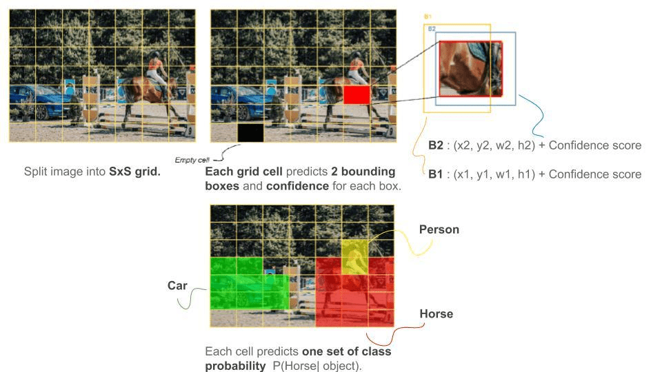
At test time, the model designates each box with its class-specific confidence score by multiplying the confidence score of each box with its respective class-conditional probabilities, these scores evaluate the probability of the class appearing in the box, and how precise the box coordinates are.
\[Pr(Class_i |Object) \times Pr(Object) \times IoU^{ truth}_{ pred} = Pr(Class_i ) \times IoU^{ truth}_{ pred}\]Network design and Training
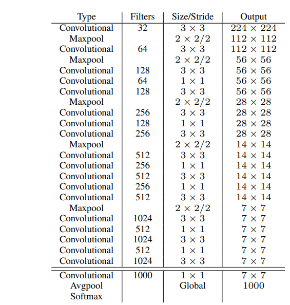
The architecture of YOLO is extremely influenced by GoogleLeNet, the network consists of 24 convolution layers for feature extraction followed by 2 fully connected layers for predicting bounding box coordinates and their respective object probabilities, replacing the inception modules of GoogleLeNet with 1x1 convolution layers to reduce the depth dimension of the feature maps.
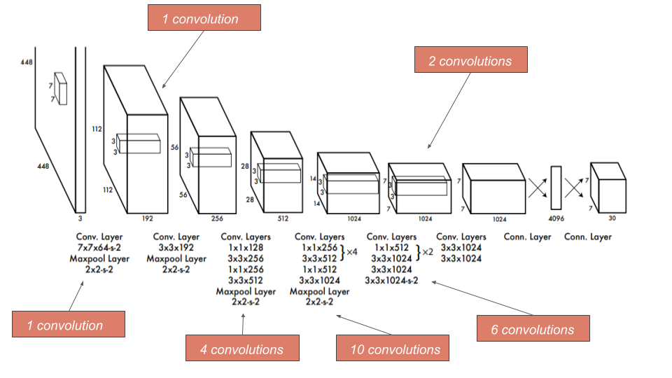
Modified figure of YOLO architetcure (source)
YOLO’s training consists of 2 stages:
-
First we pretrain the network to perform classification with 224x224 input resolution on ImageNet, using only the first 20 convolution layers followed by an average pooling and a fully connected layer.
-
Secondly we train the network for detection by adding four convolution layers and two fully connected layers. For detection we train on 448x448 resolution inputs since gradually training on higher resolution images considerably increases accuracy given that subtle visual information is more evident for detection.
Fast YOLO a relatively smaller network of 9 convolution layers, is also introduced by the authors, this over-simplified network structure contributes to an impressive speed of 155 fps, becoming the fastest detector in object detection literature, but still achieving a relatively low accuracy of 52.5 mAP.
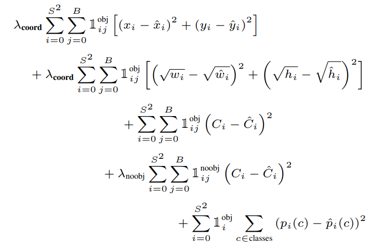
Loss function
The objective function of YOLO may look intimidating, but when broken down it is fairly understandable.
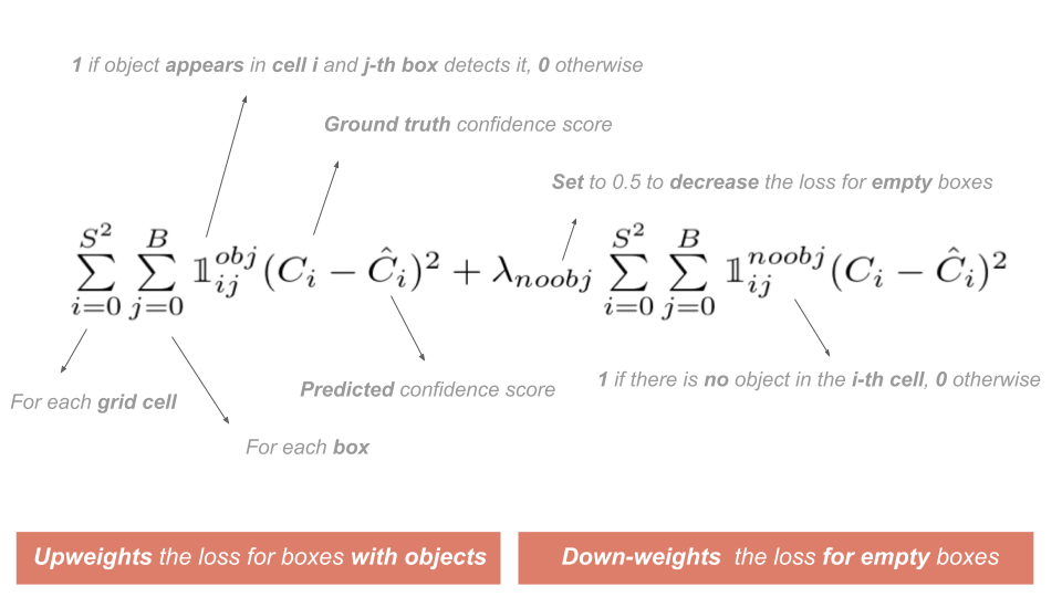
YOLO uses three-part sum-square error (SSE) . The localization loss term that penalizes the bounding box coordinates, classification loss term that penalizes class-conditional probabilities in addition to the confidence loss term.
Confidence loss. Due to the grid paradigm of YOLO, the network generates a large set of boxes that do not contain any object, so these predictor boxes get a confidence score of zero. Note that these empty boxes overpower those containing objects, thereby overwhelming their loss and gradient. To tackle this problem, we decrease the loss of low confidence predictions by setting \(\lambda_\text{noobj} = 0.5\).
To ensure that the confidence loss strongly upweights the loss of boxes that contain an object (i.e. Focus training on boxes containing an object), we set the following mask \(1^{ obj}_{ij}\)
\[\mathbb{1}_{ij}^\text{obj}= \begin{cases} 1 & \text{if } \text{ the object exists in the i-th cell and j-th box is responsible for detecting it.} \\ 0 & \text{otherwise} \end{cases}\]Similarly to down-weight the loss for empty boxes we set the mask \(1^{noobj}_{ij}\)
\[\mathbb{1}_{ij}^\text{noobj}= \begin{cases}1 & \text{if } \text{ there is no object in the i-th cell } \\ 0 & \text{otherwise} \end{cases}\]This makes the confidence loss as follows :
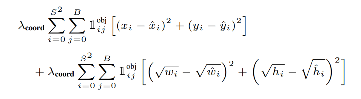
localization loss. SSE also equalizes error in large and small boxes which is not ideal either because a small deviation is more prominent in a small box than in a larger one. To resolve this, we predict the square root of height and width coordinates instead of the height and width directly.
Additionally, the loss function only penalizes the localization error for the predictor box that has the highest IoU with ground truth box in each grid cell in order to increase the loss for bounding box coordinates and focus more on detection we set \(\lambda_\text{coord} = 5\). Therefore, the localization loss becomes :
Classification loss. Finally, for the classification loss, YOLO uses sum squared error to compare the class-conditional probabilities for all classes, and to further simplify learning we want the loss function to penalize the classification error only if an object is present in the grid cell, so we set the following mask \(\mathbb{1}_i^\text{obj}\).
\[\mathbb{1}_i^\text{obj} = \begin{cases}1 & \text{if } \text{the object exist in the i-th cell } \\ 0 & \text{Otherwise} \end{cases}\]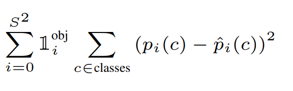
The YOLO loss function. Consequently, the loss function of YOLO is expressed as follows:
Inference
Due to its simplified and unified network structure, YOLO is fast at testing time. On Pascal VOC, YOLO predicts 98 bounding boxes per image with corresponding class probabilities.
Considering that large number of predicted boxes where multiple boxes detect the same object, we perform non-max suppression (nms) to keep only the best bounding box per object and effectively discard the others.
This is how nms works:
- First, discard boxes with low confidence score (i.e. empty boxes) with a threshold of 0.6.
For the rest, for each class :
-
Select the box with the greatest confidence score (i.e. The box that fits the object the most)
-
Then discard boxes with an IoU above a designated threshold, these boxes mostly overlap with our finest box.
By using nms, the performance of YOLO improves by 2-3% mAP.
Limitations
-
YOLO performs poorly on small objects, particularly those appearing in groups, as each grid cell predicts only B=2 bounding boxes of the same class, creating a spatial constraint that limits the number of objects predicted per grid cell.
-
Although the loss function predicts the square root of bounding box height and weight instead of height and weight directly in attempt to solve the error equalization for large and small boxes, this solution partially remedies the problem, resulting a significant number of localisation errors.
-
In addition, YOLO fails to properly detect objects of new or uncommon shapes, as it does not generalize well beyond the bounding boxes in the training set.
Major features of YOLO
-
By predicting bounding box coordinates directly from input images, YOLO treats object detection as a regression problem, unlike classifier based methods.
-
The refreshingly simple network of YOLO is trained jointly enabling 45 fps of real-time speed prediction .
-
Moreover, since it simultaneously predicts bounding boxes from the entire image across all classes, the network reasons globally about all the objects in the image.
YOLOv2
Although object detection applications have tremendously improved with latest advancements in computer vision based on deep learning, the scope of object detection is still restricted to a small set of objects, this is due to limited number of labeled datasets for detection.
The most prevailing detection dataset Pascal VOC detects 20 categories, similarly MS COCO detects 80 categories comprising thousands of to hundreds of images, while classification datasets have millions of images with hundreds of thousands of categories. This is primarily owing to the difficult task of labelling dataset for detection while user-supplied metadata such as keywords or tags associated with the image provide the job of classification effortlessly.
To close the dataset size gap between detection and classification task, the paper introduces YOLO9000, a real-time object detection system that detects over 9000 object categories, YOLO9000 leverages the massive classification dataset to correctly localize unlabeled objects for detection using a joint training algorithm on both COCO detection dataset and ImageNet classification dataset.
Furthermore, since the original YOLO model (let’s call it YOLOv1) suffers from localization errors and low recall predictions, the paper presents YOLOv2, which proposes novel and prior work-based improvements, namely SSD, to address the above constraints and further increase the speed vs accuracy trade-off.
The authors sought to make YOLO faster while performing more accurately, hence the humorous title of the paper “Better, Faster and Stronger”, thus proposing the the following improvements to achieve each of these goals :
Adjustments for a better YOLO
- Batch normalization. By adding batch normalization on all convolutional layers in YOLO, the performance improves by 2% mAP, batch norm has a regularizing effect, therefore we can remove dropout without overfitting.
-
Classifying on high resolution inputs. Yolo pretrains the classifier on ImageNet using 224x224 resolution inputs, then increases the resolution to 448x448 for detection, it requires the network time to simultaneously adjust to the new resolution input and perform the detection task. However YOLOv2 resolves this by :
-
Firstly train the classifier on 224x224 resolution on ImageNet.
-
Secondly fine tune the classifier on 448x448 resolution for 10 epochs, this make the network’s filters adjust to higher resolution inputs.
-
Then fine tune the resulting network on detection.
Fine tuning the classifier on higher resolution inputs increases accuracy by 4% mAP.
-
- Convolutional layers with anchor boxes. YOLO predicts bounding box coordinates straight from fully connected layers located on top of convolutional feature extractor layers, while SSD and Faster R-CNN predict offsets to anchor boxes.
What are anchor boxes ?
Anchor boxes (also called default boxes) are a set of predefined box shapes selected to match ground truth bounding boxes, because most of objects in the training dataset or generally in the world (e.g. person, bicycle, etc.) have a typical height and width ratio. So when predicting bounding boxes we just adjust and refine the size of those anchor boxes to fit the objects, hence the word use of offset.
The use of anchor boxes makes the learning process tremendously easier, in addition to achieving multi-scale detection by specifying anchor boxes of varying sizes.By using anchor boxes, YOLOv2 improved recall by 7% which means it increased the percentage of positive cases, however it decreased accuracy by a small margin.
But how to implement anchor boxes in YOLOv1?
Firstly remove the fully connected layers together with the pooling layer to maintain a high resolution feature map that would be suitable for tiling anchor box.
Since the most images tend to have big objects in the center, we want a single center location to predict these objects, therefore we need an odd number of locations on the feature map. To achieve this we reduce the input resolution of the network from 448x448 to 416x416 to have a single center cell.
The downsampling of convolutional layer step in YOLOv1 by a factor of 32 on the inputs of 416x416 resolution result in a 13x13 feature map.
Similar to YOLOv1, we predict the offset coordinates for each anchor box, the confidence score of the box which computes the IoU of the ground truth and predicted box, and a set of class-conditional probabilities.
-
Dimension clusters. To yield better result, instead of hand picking the prior boxes dimensions, we select the finest priors by running K-means clustering algorithm on the training set to find the top K prevalent bounding boxes.
To find the nearest centroid to each ground truth bounding box, we do not use the usual Euclidean distance as the distance metric because it generates errors for large boxes, but we are looking for priors that have good IoU score with ground truth boxes regardless of box size, so we use the following distance metric :
\(d(box, centroid) = 1 − IoU(box, centroid)\)
For different K cluster values, we find that K=5 is the best value because it offers a good trade-off between the complexity of the model and high recall (i.e. percentage of positive cases).
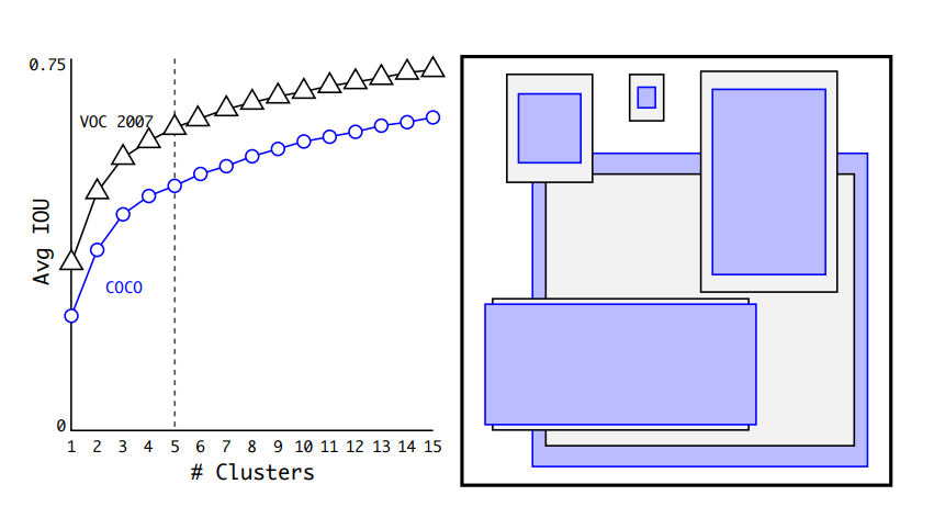
Left: For different numbers of clusters k we plot the average IoU score, k=5 offers a good trade-off for model complexity vs recall. Right: The 5 anchor box shapes selected for COCO in blue and Pascal VOC 2007 in gray color (source)
-
Direct location prediction. Region proposal network (RPN) predicts anchor box offsets, offsets that are not constrained to a specific location and could end up in any part of the image, regardless of what location predicted this box. Using this strategy on YOLOv1 led it to be unstable during training, as the prediction is not unconstrained, it requires a long time for the model to predict sensible offsets.
Therefore, for each anchor box YOLOv2 predicts bounding box coordinates relative its grid cell location, for this purpose we use a logistic activation function to output coordinates within a range of [0,1].
To specify the corresponding grid cell for each prediction :
-
First, we define the grid cell that the top left corner of the anchor box belongs to \((c_x, c_y)\), the anchor is of size \((p_w, p_h)\).
-
Secondly we predict offsets to this anchor \((t_x, t_y, t_w, t_h)\) along with the \(t_o\) confidence score.
-
In order to constrain the predicted box to its corresponding grid cell, we bound the box’s center coordinates to the center location by using using the sigmoid function σ.
This final predicted box is of \((b_x, b_y, b_w, b_h)\) parameters :
\(\begin{aligned} b_x &= \sigma(t_x) + c_x\\ b_y &= \sigma(t_y) + c_y\\ b_w &= p_w e^{t_w}\\ b_h &= p_h e^{t_h}\\ \text{Pr}(\text{object}) &\cdot \text{IoU}(b, \text{object}) = \sigma(t_o) \end{aligned}\) -
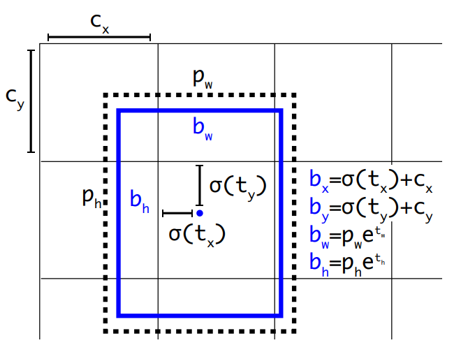
This approach improves accuracy by 5%.
-
Fine-Grained Features. As mentioned earlier, the modified YOLO outputs a 13x13 resolution feature map, which does a sufficient job at detecting large objects, but it comes short when detecting small-scale objects as we get deeper in the network due to the loss of their semantic features.
That being said, using higher-resolution feature maps helps the network detect objects of different scales, so YOLOv2 adapts this approach, but instead of stacking a layer of high-resolution on top of the convolution layers, we concatenate the features of a 26x26 resolution layer with the low resolution features along the channels, making the 26x26x512 feature map a 13x13x2048 feature map, similar to identity mappings in ResNet. This approach improves the model by a modest 1%.
-
Multi-Scale Training. Since our network consists only of convolutional and pooling layers, not fully connected layers, we can train the network on different input sizes so that it can be robust to different input sizes, thus detecting well on different resolutions.
Therefore, during training for every 10 batches, the network randomly chooses a new image size, since our model downsamples by a factor of 32, the chosen sizes should be a multiple of 32.
Comparing performance
The following plot is created to evaluate the performance of YOLOv2 trained on VOC 2012 with different input dimensions against its counterpart detectors:
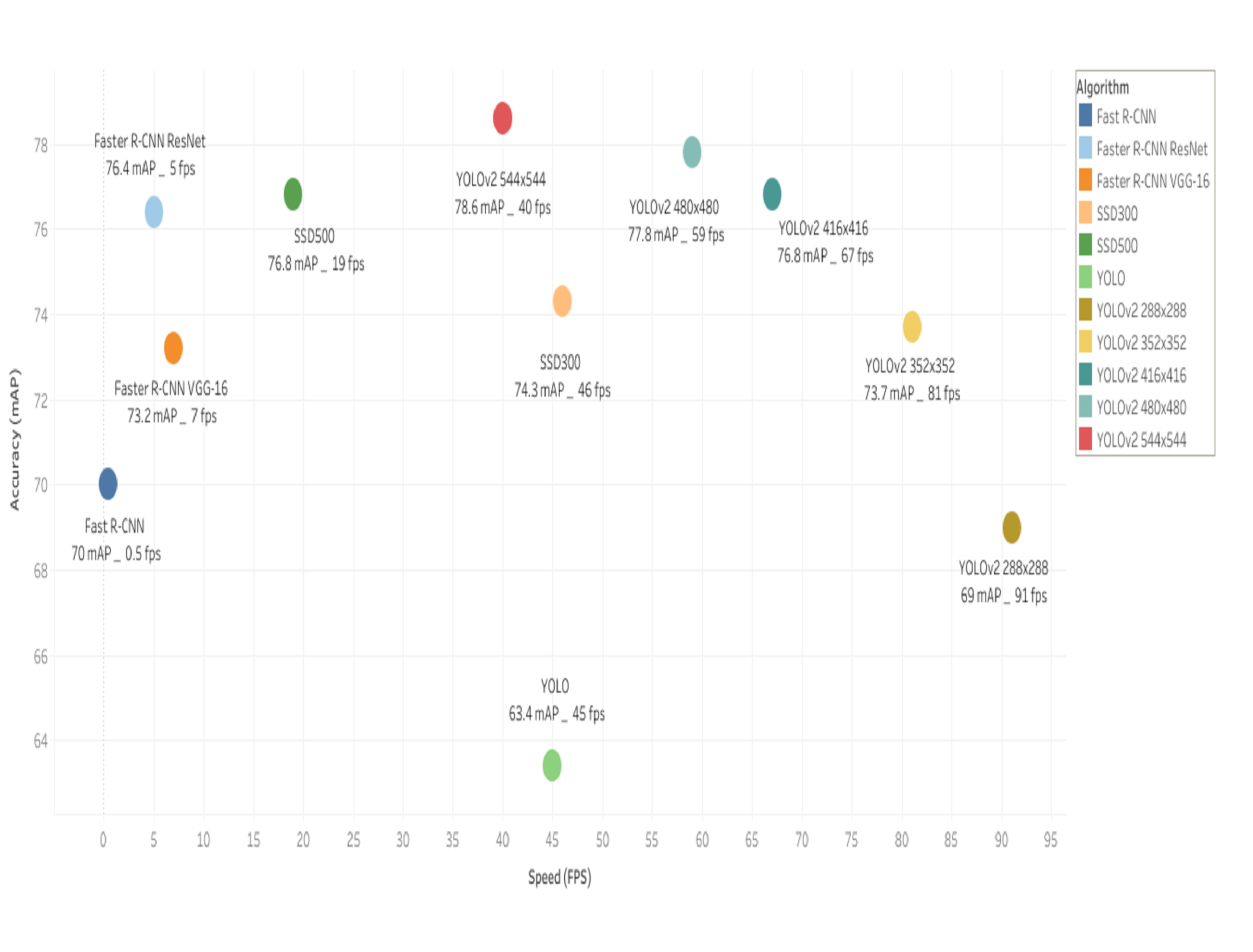
Accuracy and speed on Pascal VOC 2007
-
It can be seen that YOLOv2 runs faster with smaller resolution inputs outperforming other detection methods while attaining a competitive accuracy to Fast R-CNN.
-
Furthermore, at a high resolution of 544x544 YOLOv2 is more accurate than all prior methods while running above real-time speed, namely faster than the R-CNN family and SSD500.
Making YOLO faster with Darknet-19
Most of object detection methods use VGG-16 as a base feature extractor, it yields good results in terms of accuracy nonetheless, it has a complex architecture, it requires 30.69 billion floating point operations to process a single image at a low resolution, which is undoubtedly a concern when dealing with low latency applications.
While YOLOv1 leverages GoogeLeNet architecture which is relatively fast with 8.52 billion operations for a forward pass, it falls short in terms of accuracy achieving 88.0% mAP on ImageNet compared to 90.0% mAP with VGG-16.
In YOLOv2, the author sought to maximize performance by developing a custom network that is both accurate and fast to support applications that require near real-time speed such in self driving cars. This is where Darknet-19 is presented, Darknet-19 achieves 91.2% accuracy, but most importantly, the processing of an image requires only 5.58 billion floating point operations.
Darknet-19 design. Darknet is consists of 19 convolution layers mainly using 3x3 filters with 5 max-pooling layers, as well as using global average pooling for predictions and using 1x1 filters to reduce the depth channels between the 3x3 convolutions.
We use batch normalization to ensure stability during training and allow faster convergence.
Darknet-19 network design (source)
Training for classification & detection. According to the above mentioned training strategy, YOLOv2 trains the classifier on ImageNet with low resolution input of 224x224 for 160 epochs, then fine tunes it on high input resolution of 448x448 for 10 epochs. To fine tune the resulting network for detection, we substitute the last three convolution layers with 3x3 convolutional layers with 1024 filters, followed by a final 1x1 convolution.
Since we want the network to output predictions for 5 anchor, for each anchor predict 4 bounding box coordinates, confidence score and 20 class probabilities, we use (4+20) x 5=125 filters. The network is trained for 160 epochs, it starts with a learning rate of \(10^-3\), then the learning rate is divided by 10 for every 60 and 90 epochs.
Making YOLO stronger with YOLO9000
In addition to the above-mentioned improvements with YOLOv2, the paper also presents YOLO9000, a real-time system that detects more than 9000 objects categories by combining COCO’s detection dataset with ImageNet’s classification dataset. YOLO9000 learns detection-labeled data about the bounding box coordinate prediction and obje ctness score, and from the classification-labeled data, it learns new categories of deeper range to expand the number of categories that the model can detect.
But how does this work?
We could use a softmax function to output the probability distribution across different categories, but the softmax assumes that the classes are mutually exclusive, which is not the case in our scenario as COCO has more generic categories such as “dog” and ImageNet has more specific categories like dog breeds e.g. “Norfolk terrier” and “Yorkshire terrier”. However, If we consider the task to be one of multi-label classification, by using a sigmoid function we completely discard COCO’s data structure with mutually exclusive classes.
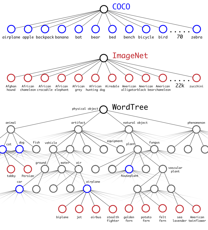
On the other hand, it’s not wise to assume a flat structure to the labels, as the classes are hierarchically structured. That’s why we use WordNet, a lexical database that groups words into synonym sets called synsets and structures their semantic relationships in a tree where sysnets are on the same level and hyponyms are lower level nodes in the lower level to the current node.
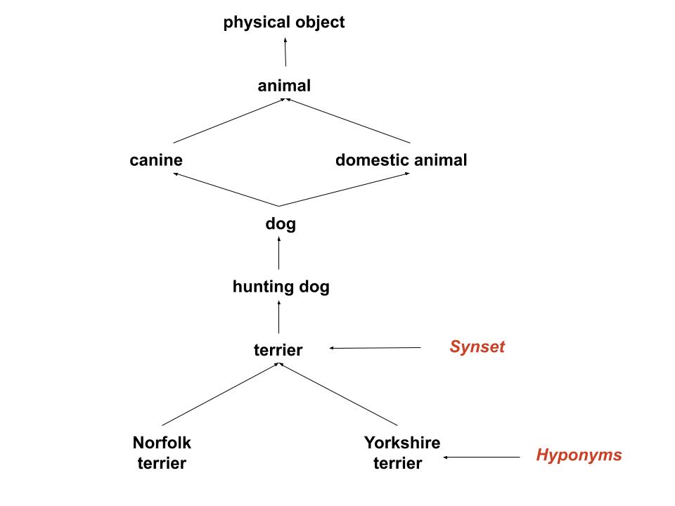
Small subset of the graph for illustration purposes only.
However, to simplify the problem we don’t use the full graph structure of WordNet, we just want ImageNet’s categories so we construct WordTree, a hierarchical tree that only includes WordNet’s extracted ImageNet labels.
But how do we perform classification with WordTree?
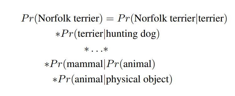
First, we compute the probability of an object being in an image via the law of total probability, by computing the conditional probability of the specific node of the object given its synset following the path to the root node and multiply the conditional probabilities. We assume that the image contains an object so \(P_r(\text{physical object})=1\).
We also consider the intermediate nodes to train Darknet-19 on WordTree, which extends the label range from 1000 ImageNet classes to 1369.
During training, the network propagates the tree so that a node category can also be labeled as the categories in the path to the root node, e.g. “Norfolk terrier “ can also be labeled as “terrier” and “hunting dog”, etc. This way even if the model is uncertain of the breed of the dog, it can always bounce back by predicting it as a “dog”.
Furthemore, in order to compute these conditional probabilities, the model outputs a 1369 vector on which we apply a softmax function to predict probability distributions, but we do not apply it as usual over the entire vector, we use multiple softmax over the synsets which are hyponyms of the same concept.
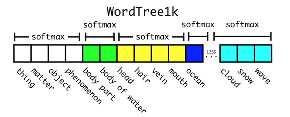
Training Darknet-19 on WordTree with 1369 labels achieves top-1 accuracy of 71.9% (i.e. considering only the highest prediction) and top-5 accuracy of 90.4% (i.e. considering the top 5 predictions).
Now after training on WordNet built on ImageNet, we combine both datasets ImageNet and COCO with WordTree by simply mapping the labels to synsets in the WordTree hierarchy.
Combining ImageNet and COCO datasets using WordTree hierarchy (source)
The network backpropagates the loss as usual for detection images, however the loss only backpropagates at or above the corresponding label level for classification images. For instance, if the corresponding label is “dog”, we don’t want the error to backpropagate to the level of the dog breed since we don’t have that information.
To evaluate the model, we use ImageNet detection challenge categories that shares 44 object categories with COCO, leaving 156 object classes that the model did not train on for detection. On the 156 unseen labeled data for detection, the model achieves 16 mAP and 19.7 mAP on the entire testing data.
Generally YOLO9000 generalizes well on objects that are sub-classes of categories that the model learned in the training set, such as new animal species, but fails to model categories such as clothing mainly because COCO has no category of clothing type.
Main point
YOLO9000 is certainly an innovative approach that bridges the gap between the scope of object classification and detection systems, by leveraging the large amount of classification data we already have to produce a more robust, comprehensive detection system.