
Object detection metrics serve as a measure to assess how well the model performs on an object detection task. It also enables us to compare multiple detection systems objectively or compare them to a benchmark. Accordingly, prominent competitions such as PASCAL VOC and MSCOCO provide predefined metrics to evaluate how different algorithms for object detection perform on their datasets.
Now you may have stumbled upon unfamiliar metric terms like AP, recall, precision-recall curve or simply stated in a research paper that the model has high sensitivity. The use of multiple metrics can be often confusing. Therefore, in this post we explain the main object detection metrics and the interpretation behind their abstract notions and percentages. As well as how to know if your model has a decent performance and if not what to do to improve it.
- Key notions
- Interpretations
- Precision - recall and the confidence threshold
- Precision x Recall curve
- Average Precision
- Mean average precision (mAP)
- Average recall (AR)
- Metrics chosen for popular competitions
Key notions
Since the classification task only evaluates the probability of the class object appearing in the image, it is a straightforward task for a classifier to identify correct predictions from incorrect ones. However, the object detection task localizes the object further with a bounding box associated with its corresponding confidence score to report how certain the bounding box of the object class detected.
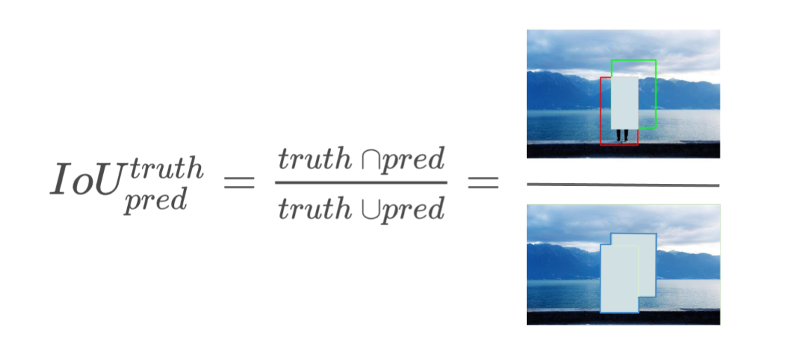
Therefore to determine how many objects were detected correctly and how many false positives were generated (will be discussed below), we use the Intersection over Union (IoU) metric.
Intersection over Union (IoU)
Intersection over Union, also referred to as the Jaccard Index, is an evaluation metric that quantifies the similarity between the ground truth bounding box (i.e. Targets annotated with bounding boxes in the test dataset) and the predicted bounding box to evaluate how good the predicted box is. The IoU score ranges from 0 to 1, the closer the two boxes, the higher the IoU score.
Formally, the IoU measures the overlap between the ground truth box and the predicted box over their union.
Predictions: TP - FP - FN
By computing the IoU score for each detection, we set a threshold for converting those real-valued scores into classifications, where IoU values above this threshold are considered positive predictions and those below are considered to be false predictions. More precisely, the predictions are classified into True Positives (TP), False Negatives (FN), and False Positives (FP).
Below is the case of a true positive prediction on the left, the two cases in the center of a false positive prediction, and the false negative prediction on the left.
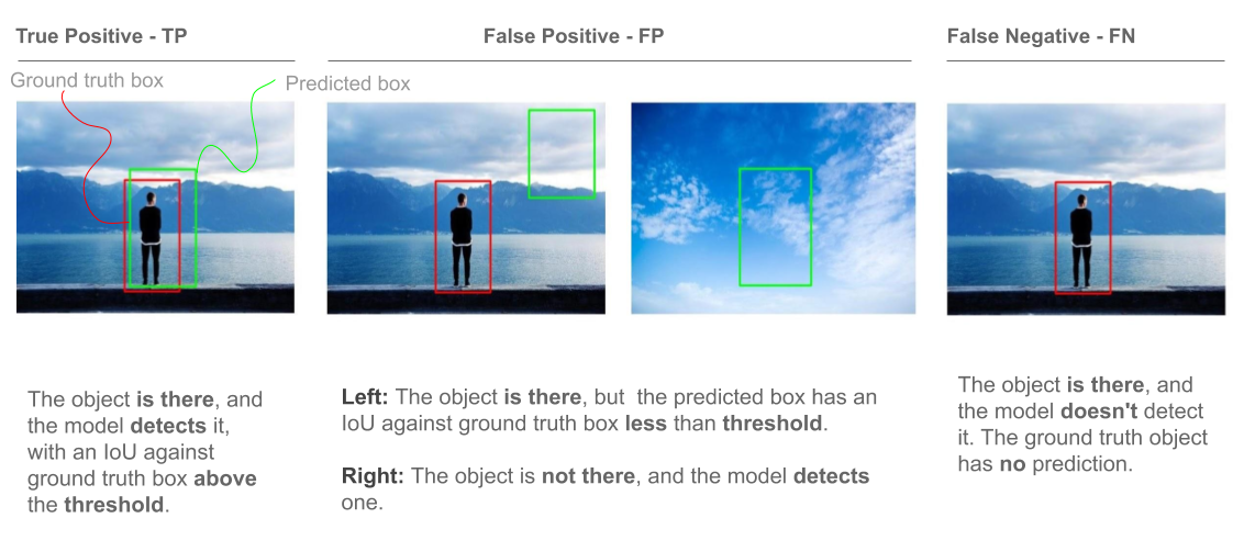
You may note that I did not mention True Negative predictions (TN), on the grounds that it describes the situation where empty boxes are correctly detected as “non-object”. In this scenario, the model would evidently identify thousands of empty boxes which adds little to no value to our algorithm. Furthermore, in calculating object detection metrics, which we will address soon, false negatives are not essential.
Why accuracy is not a reliable metric?
- Accuracy : is the percentage of correctly predicted examples out of all predictions, formally known as
The accuracy result can be very misleading when dealing with class imbalanced data, where the number of instances is not the same for each classes, as It puts more weight on learning the majority classes than the minority classes.
In detection datasets, class distribution is considerably non-uniform. For instance, in the renowned Pascal VOC 2007 dataset, the “person” class is by far the most frequent one with 9,218 object instances, whereas the ‘dining table’ class is of 421 instances.
Precision
Precision is the the probability of the predicted bounding boxes matching actual ground truth boxes, also referred to as the positive predictive value.
Precision scores range from 0 to 1, a high precision implies that most detected objects match ground truth objects. E.g. Precision = 0.8, when an object is detected, 80% of the time the detector is correct.
You may want to consider applying hard negative mining To improve low precision (i.e. include negative examples in training) since the model suffers from high false positives.
Recall
Recall is the true positive rate, also referred to as sensitivity, measures the probability of ground truth objects being correctly detected.
Similarly, recall ranges from 0 to 1 where a high recall score means that most ground truth objects were detected. E.g, recall =0.6, implies that the model detects 60% of the objects correctly.
Interpretations
- High recall but low precision implies that all ground truth objects have been detected, but most detections are incorrect (many false positives).
- Low recall but High precision implies that all predicted boxes are correct, but most ground truth objects have been missed (many false negatives).
- High precision and high recall, the ideal detector has most ground truth objects detected correctly.
Note that we can evaluate the performance of the model as a whole, as well as evaluating its performance on each category label, computing class-specific evaluation metrics.
To illustrate how recall and precision are calculated, let’s look at an example of a object detection model. Below are images of objects where those on the left depict the ground truth bounding boxes, and those on the right represent the predicted boxes. We set the IoU threshold at 0.5.
Bear in mind that the predictions are individually calculated for each class.
-ec90cda7-f58f-4259-9887-b4fde66c6c33.png)
How predictions work:
- When multiple boxes detect the same object, the box with the highest IoU is considered TP, while the remaining boxes are considered FP.
- If the object is present and the predicted box has an IoU < threshold with ground truth box, The prediction is considered FP. More importantly, because no box detected it properly, the class object receives FN, .
- If the object is not in the image, yet the model detects one then the prediction is considered FP.
- Recall and precision are then computed for each class by applying the above-mentioned formulas, where predictions of TP, FP and FN are accumulated.
Let’s calculate recall and precision for the ‘Person’ category:
Recall \(= \frac{TP}{TP + FN}\) \(= \frac{1}{1+1}\) \(=\) 50%
Precision \(= \frac{TP}{TP + FP}\) \(= \frac{1}{1+2}\) \(=\) 33%
Now if you’re not satisfied with those results, what can you do to improve the performance? This is where the confidence threshold comes into the picture.
Precision - recall and the confidence threshold
When optimizing your model for both recall and precision, it is unlikely that an object detector will yield both peak recall and precision on an object class at all times, mainly because of a trade-off between the two metrics. This trade-off depends on the confidence threshold. Let’s see how this works:
The object detector predicts bounding boxes, each associated with a confidence score. The confidence score is used to assess the probability of the object class appearing in the bounding box. Accordingly, we set a threshold to turn these confidence probabilities into classifications, where detections with a confidence score above the predetermined threshold are considered true positives (TP), while the ones below the threshold are considered false positives (FP).
When choosing a high confidence threshold, the model becomes robust to positive examples (i.e. boxes containing an object), hence there will be less positive predictions. As a result, false negatives increase and false positives decrease, this reduces recall (the denominator increases in the recall formula) and improves precision (denominator decreases in the precision formula). Similarly, further lowering the threshold causes the precision to decease an recall to increase.
Therefore, the confidence threshold is a tunable parameter where by adjusting it we can define TP detections from FP ones, controlling precision and recall, thereby determining the model’s performance.
Accordingly, for the above example in the images, in order to reduce false positive prediction, consider increasing recall by increasing the confidence threshold.
Precision x Recall curve
Another metric that summarizes both recall and precision and provides a model-wide evaluation is the precision x recall curve. Since both metrics do not use true negatives, the precision x recall curve is a suitable measure to assess the model’s performance on imbalanced datasets.
Furthermore, Pascal VOC 2012 challenge utilizes the precision x recall curve as a metric in conjunction with average precision which will be addressed later in this post.
As the name implies, the precision x recall curve plots recall on the x-axis and precision on the y-axis, where each point in the curve represents recall and precision values for a certain confidence value.
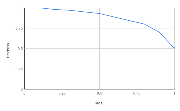
An ideal model is depicted to have an optimal point closer to [1.0, 1.0].
When recall increases, an ideal model would have high precision, otherwise the model performs poorly. In this situation, consider increasing recall to correctly detect all ground truth objects by reducing the confidence threshold.
On the other hand when comparing multiple models, the one with highest curve in the precision x recall plot is considered the better performer.
Nevertheless, due to the trade-off between recall and precision, the curve can be noisy and have a particular saw-tooth shape that makes it difficult to estimate the performance of the model and similarly difficult to compare different models with their precision x recall curves crossing each other. Therefore we estimate the area under the curve using a numerical value called Average Precision.
Average Precision
Average precision (AP) serves as a measure to evaluate the performance of object detectors, it is a single number metric that encapsulates both precision and recall and summarizes the Precision-Recall curve by averaging precision across recall values from 0 to 1, let’s clarify this in detail:
11-point interpolated average precision
AP averages precision at a set of 11 spaced recall points (0, 0.1, 0.2, .. , 1) where we interpolate the corresponding precision for a certain recall value r by taking the maximum precision whose recall value \(\widetilde{r}> r\). In other words, take the maximum precision point where its corresponding recall value is to the right of r. In this case, Precision is interpolated at 11 recall levels, hence the name 11-point interpolated average precision.
This is particularly useful as it reduces the variations in the precision x recall curve. This interpolated precision is referred to as \(p_{interp}(r)\).
\[AP = \frac{1}{11}\sum_{r\in\left\{0,0.1,0.2,...,1\right\}}^{} p_{interp}(r)\]where
\[p_{interp}(r) =\max_{\widetilde{r} > r} p(\widetilde{r})\]Now for the above example, let’s calculate 11-point interpolated AP:
-7d3272db-e4e0-4f69-8aff-128f07ed6068.png)
Precision is interpolated with the maximum precision point to the right at recall level 0.3. This is indicated by the orange line in the graph.
Similarly, this approach is applied to all of 11 recall values (0,0.1,0.2,…,1). In our particular situation, recall levels start with 0.2, nevertheless the strategy remains the same.
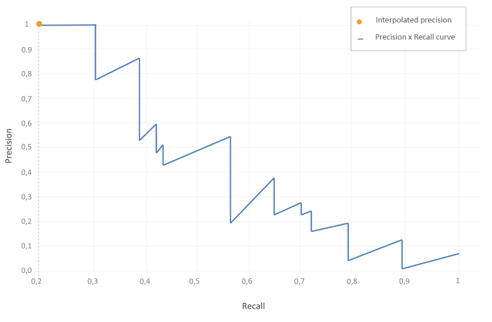
Now to compute AP, we average all of the interpolated precision points.
\[AP = \frac{1}{11} \sum_{r\in\left\{0,0.1,0.2,...,1\right\}}^{}p_{interp}(r)\] \[AP = \frac{1}{11} (1 + 0.87+ 0.6 + 0.54 + 0.38 + 0.25 + 0.13 + 0.08)\]\(AP = 35\) %
All point average precision
Prior to 2010, the Pascal VOC competition used 11-point interpolation, but ultimately changed the approach to computing AP by using all recall levels instead of only using 11 recall points to effectively compare detection algorithms with low AP scores.
-848db820-1379-456f-bad8-8e45ea562fd0.png)
Since all recall points are now included, the area under the curve (AUC) can be closely estimated as AP, hence we can calculate AP by directly computing the area under the curve (AUC). AUC is the sum of all the separate areas under the curve, where a separate area is defined by a drop of precision at a certain recall r.
Consequently, for our example, we are dividing the area under the curve to 10 areas.
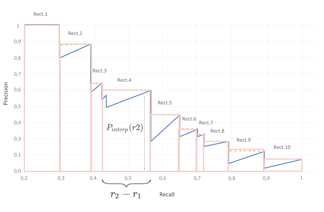
This translates mathematically into the following:
where
\[p_{interp}(r_{n}) =\max_{\widetilde{r} > r_{n}} p(\widetilde{r})\]Now AP is the total sum of the 10 rectangle areas under the curve, where:
\(AP =\) Rect.1 + Rect.2 + Rect.3 +Rect.4 + Rect.5 + Rect.6 + Rect.7 + Rect.8 + Rect.9 + Rect.10
\(AP =\)(0.3 - 0.2) x 1 + (0.38 - 0.3) x 0.88 + (0.42 - 0.38) x 0.6 + (0.56 - 0.42) x 0.54 + (0.65 - 0.56) x 0.38 + (0.7 - 0.65) x 0.28 + (0.72 - 0.7) x 0.25 + (0.79 - 0.72) x 0.2 + (0.89 - 0.79) x 0.14 + (1- 0.89) x 0.08
\(AP =\) 0.1 + 0.0704 + 0.024 +0.0756 + 0.0342 + 0.014 + 0.005 + 0.014 + 0.014 + 0.0088
\(AP =\) 36%
Mean average precision (mAP)
Now that we understand AP, mean average precision (I know when it’s laid out it sounds quite absurd) is a refreshingly simple matter. In essence, if the dataset contains N class categories, the mAP averages AP over the N classes.
In addition, PASCAL VOC challenge uses mAP as a metric with an IoU threshold of 0.5, while MS COCO averages mAP over different IoU thresholds (0.5, 0.55, 0.6, 0.65, 0.7, 0.75, 0.8, 0.85, 0.9, 0.95) with a step of 0.05, this metric is denoted in papers by mAP@[.5,.95]. Therefore, COCO not only averages AP over all classes but also on the defined IoU thresholds.
Note that mAP and AP are often used interchangeably, this is the case with COCO competition. According to their official website:
’ AP and AR are averaged over multiple Intersection over Union (IoU) values. Specifically we use 10 IoU thresholds of .50:.05:.95. This is a break from tradition, where AP is computed at a single IoU of .50 (which corresponds to our metric \(AP^{IoU}=.50\). Averaging over IoUs rewards detectors with better localization. ‘
By optimizing AP or AR (discussed next) over multiple IoU threshold values, the model penalizes poor localization and optimizes for good localization. Simply because the localization accuracy is evaluated on the basis of the IoU between the ground truth and the predicted box, this is the optimal strategy to be used for detection applications that require high localization, such as self driving cars or medical imaging.
Average recall (AR)
Rather than computing recall at a particular IoU, we calculate the average recall (AR) at IoU thresholds from 0.5 to 1 and thus summarize the distribution of recall across a range of IoU thresholds.
We only average recall over IoU thresholds from [0.5, 1] because the detection performance correlates with recall at thresholds above 0.5, where at 0.5 boxes loosely localize the objects and at an IoU of 1 the objects are impeccably localized.
Therefore, if you want to optimize your model for high recall and accurate object localization, you may want to consider average recall as an evaluation metric.
Average recall describes the area doubled under the Recall x IoU curve. The Recall x IoU curve plots recall results for each IoU threshold where IoU ∈ [0.5,1.0], with IoU thresholds on the x-axis and recall on the y-axis.
Consequently, this translates mathematically into :
\(AR = 2 \int_{0.5}^{1} recall(IoU) \text{d}IoU\)
Similarly to mAP, mAR is the average of AR over the number of classes within the dataset.
Metrics chosen for popular competitions
The COCO Object Detection Challenge : evaluates detection using 12 metrics where:
-
mAP (interchangeably referred to in the competition by AP) is the principal metric for evaluation in the competition, where AP is averaged over all 10 thresholds and all 80 COCO dataset categories. This denoted by AP@[.5 : .95] or AP@[.50: .05: .95] incrementing with .05. Hence, a higher AP score according to the COCO evaluation protocol indicates that detected objects are perfectly localized by the bounding boxes.
-
Additionally, COCO individually evaluates on AP at 0.5 and 0.75 IoU thresholds, this is denoted by AP@.50 or AP\(^{IOU=0.50}\) and AP@.75 or AP\(^{IOU=0.75}\) respectively.
- Since COCO dataset contains small objects more than large ones, the performance is evaluated on AP in distinct object dimensions where:
- AP \(^{small}\) for small objects of area less than 32 \(^2\).
- AP \(^{medium}\) for medium object of area 32 \(^2\) < area < 96 \(^2\).
- Finally, AP \(^{large}\) for large objects with area greater than 96 \(^2\).
The object area is defined by the number of pixels in the object mask provided for the object segmentation task in COCO competition.
-
Similarly, COCO evaluates the algorithms on mAR (mAR is referred to by AR) across scales with AR \(^{small}\), AR \(^{medium}\) and AR \(^{large}\).
- Furthermore, COCO uses an additional metric which bases the AR evaluation on the number of detections per image number, specifically AR \(^{max=1}\) given 1 detection per image, AR \(^{max=10}\) for 10 detections per image and AR \(^{max=100}\) for 100 detections per image.
The PASCAL VOC Challenge : The Pascal VOC evaluation is based on two metrics, the precision x recall curve and average precision (AP) computed at the 0.5 single IoU threshold.
The Open Images Challenge : To evaluate the result of object detection models, the Google Open Image challenge uses mean Average Precision (mAP) over their 500 classes in the dataset at an IoU threshold of 0.5.