Evolution of object detection algorithms leading to SSD

Classic object detectors are based on sliding window approach (DPM), which is computationally intensive due to the exhaustive search but is rapidly rendered obsolete by the rise of region proposals with (R-CNN, Fast R-CNN), this approach introduces a selective search algorithm for finding potential objects, performs relatively better, but has its constraints, since the search algorithm is a decoupled process from training it would generate false positives and forward them to training, this combined with the complex pipeline makes it computationally expensive as well as slow with 0.4 frames per second (fps) for Fast R-CNN.

Faster-RCNN solves the issue of disjoint pipeline by replacing the external region proposal algorithm with an embedded Region Proposal Network (RPN) which makes it a unified network, achieving 73.2 mAP on Pascal VOC2007 test set, but remaining considerably slow for real-time detection applications with 7 fps.

The next significant improvement in the history of object detection was to drop region proposals altogether and predict bounding box coordinates and confidence class scores directly from the image, one stage detectors, this structural simplicity enables real-time predictions. Introducing You Only Look Once (YOLO) a simplified network processing 21 fps and achieving an accuracy of 66.4 mAP on Pascal VOC2007, you may notice that by increasing speed we risk reducing the accuracy of the detector, this reframes the detection question as how the speed vs accuracy trade-off can be further improved.

This is where SSD is introduced performing faster namely to YOLO with 46 fps and a competitive accuracy to Faster-RCNN with 74.3 mAP.

In this post I explain the inner workings of SSD single shot detector and its main contributions to faster and more accurate performance even with low resolution input images.

Network design

Single Shot Detector (SSD) uses a unified two-part network, the base network leveraging a pre-trained VGG16 network on ImageNet, truncated before the last classification layer to extract high level features, then converting FC6 and FC7 to convolutional layers.

Next SSD extends this base network by adding auxiliary structure of convolution feature layers of progressively decreasing resolutions Conv8_2, Conv9_2, Conv10_2 and Conv11_2.

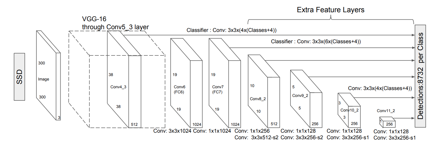
SSD architecture (source)

Forward pass workflow

The base network processes the input image to extract higher level features, it then passes through the multi-scale feature maps.

For each of the following feature maps : conv4_3, conv7 , conv8_2, conv9_2, conv10_2, and conv11_2 :

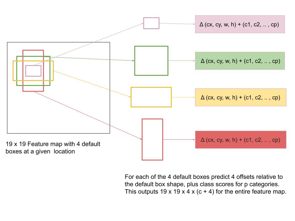
SSD sets K defaults boxes (e.g. 6) across each cell of the feature map of different scales and aspect ratios in a convolutional manner. The default boxes are pre-selected boxes from the training set to match the ground-truth bounding boxes.

Using default boxes significantly facilitates the regression task since the network predicts bounding boxes from priors that are comparable to objects in the training set rather than learning them from scratch.

SSD then passes a 3x3 filter over the feature map, and for each default box, this filter simultaneously predicts 4 bounding box coordinates relative to the default box ∆(cx, cy, w, h), i.e. offsets to the default box to better fit the ground truth box, additionally for each default box the filter outputs confidence scores for all object categories (c1, c2, · · · , cp), this is processed simultaneously, hence the name part single shot.

Default boxes and multi-scale feature maps

The reason SSD predicts offsets and confidence scores over multiple feature maps of varying resolutions is to be able to detect objects of different scales, more precisely, lower resolution feature maps detect larger objects in the image, this is partially due to the fact that semantic features of small-scale object are lost in these upper layers. As a case in point, the 8 x 8 feature map (b) detects the cat in image (a), the smaller object, while the lower resolution feature map of 4 x 4 (c) detects the larger object, the dog.

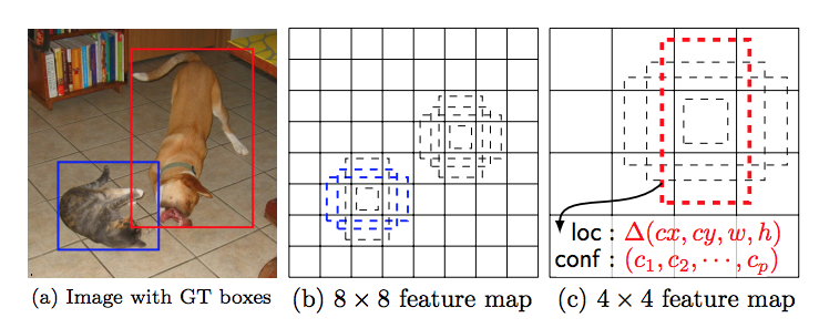
(source)

Some methods process the input image multiple times, with different sizes each time to detect objects of different scales, however SSD achieves the same purpose by using feature maps of different resolutions while sharing parameters for all object scales and not being as computationally intensive.

Small deeper resolution feature maps detect high-level semantic features where small-scale object features are lost, and since SSD uses progressively decreasing feature map resolutions, it performs worse on small objects, however increasing the input image size particularly improves the detection of small object.

Furthermore, SSD sets K default boxes of different scale and aspect ratio over every location of different feature maps to systematically discretize the search space in the image for possible objects of different shapes.

Training

For the sake of comprehensiveness, before covering the SSD objective function, I discuss the training process because the former is strongly linked to a matching strategy used in training, so kindly bear with me.

Matching strategy

SSD seek to simplify the learning process during training by selecting the best default boxes that overlap most with each ground truth box instead of choosing the best one, then train the network accordingly, but what is the matching strategy used by SSD?

For each ground truth box, SSD selects the best default box that most overlap with this specific ground truth box by finding the one that has the highest IoU (intersection over union), also called the Jaccard index.

1. For each ground truth box :

• Compare the ground truth box to default boxes and match it to the default box that obtains the highest IoU.

In addition, SSD takes another step to simplify learning:

2 . For each default box :

• Compare the default box to ground truth boxes, keep those that have an IoU > 0.5.

Considering the large number of default boxes that SSD sets over multiple feature maps, after the above-mentioned matching strategy, the unmatched boxes would be of large number, so how does SSD handle these unmatched boxes?

This brings us to the next section where hard negative mining is introduced.

Hard negative mining :

SSD mines the unmatched default boxes as negatives examples , which are background images, and forwards them to training to make the classifier more robust, however this creates an overwhelming number of negative examples that creates a class imbalance, where the model learns the background images more than the more complex categories of positive objects.

Nevertheless, instead of using all negative examples, we can select only the best ones for training :

Sort the examples in ascending order by their individual background confidence loss (i.e. individual cross entropy loss), then forward only the top ones for training, i.e. the negative examples of high confidence score, the ratio for each training batch is 3 negatives for 1 positive example.

Data augmentation

In addition to training on images with original input size, SSD samples patches that must overlap with ground truth boxes according to a Jaccard index of (0.1, 0.3, 0.5, 0.7, 0.7, 0.9) to systematically select object-containing patches, additionally SSD samples few more patches randomly, these patches create a “zoom in” effect. All of the patches mentioned are then resized to a fixed size (e.g. 300 x 300 for SSD300), flipped horizontally and underwent some photogenic distortions (Random brightness, contrast, saturation, etc).

This overly extensive sampling strategy considerably improves the performance of the model with a low resolution input of 300x300 by 8.8 mAP on Pascal Voc2007 test set.

Loss Function

Now, addressing the training objective , SSD uses Smooth \(L1\) loss to quantify the difference between the predicted box \(l\) and ground truth box \(g\) parameters \((cx, cy, h, w)\) where \((cx,cw)\) indicate the center of the offsets to default box \(d\) and \(h\) and \(w\) denotes its height and width respectively. The SSD paper along with Fast R-CNN and Faster R-CNN chose \(L1\) loss to be their localization loss because it’s more robust to outliers than \(L2\) loss.

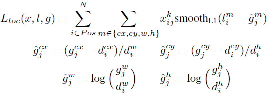
Localization loss (source)

\(\mathbb{x}{ij}^\text{p}\) indicates the \(j\)-th matched ground truth box to the \(i\)-th default box for category \(p\), \(\mathbb{x}{ij}^\text{p}\) = 1 if there is a match according to the above-mentioned matching strategy and 0 otherwise, this makes the loss focus on the matched boxes and discard the others then train the model accordingly.

Additionally, the confidence loss is a cross entropy loss over \(c\) categories :

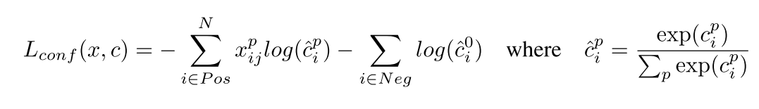
Confidence loss (source)

The final loss objective is expressed as :

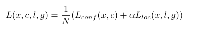
Final SSD loss (source)

The localization loss could be greater than the classification loss, therefore the network would focus more on learning the localization task than the one of classification , so we add a weighted term \(\alpha\) to balance the losses so that the model would focus on learning both tasks, and N is the number of matched default boxes.

Inference time

Taking into account the large number of boxes produced by SSD, boxes with confidence score lower than 0.01 are discarded, these are empty boxes, it then proceeds to perform non-max suppression (nms). if multiple boxes detect the same object, nms only keeps the best box per object.

Here is how it operates, for each class, nms selects the box with the highest confidence score and discards the remaining that overlap the most with this box, this is to keep only the best box per object, it uses an IOU>=0.45 threshold.

The first filtering process combined with nms results in minimizing the number of boxes per image to 200.

Performance analysis

• To further evaluate the effect of different default box shapes on performance, Wei Liu et al removed default boxes with 1/3 and 3 aspect ratios, resulting in a reduced performance of 0.6 %, and further removal of boxes with 1/2 and 2 aspect ratios reduce the performance by 2.1 %.

• To investigate the effect of using different-resolution feature layers, Wei Liu et al progressively removed each multi-scale layer and inspected the effect of each layer on detection accuracy while preserving the number of default boxes by moving the boxes of the removed layer to the remaining layers and adjusting their scales to fit the tiling of default boxes. The table below demonstrates the result of the experiment :

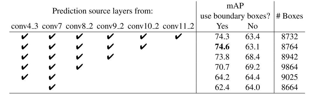
Effect of using different feature layers on SSD performance (source)

Analysis of the above table shows that only using conv7 layer decreased accuracy by a great margin of 11.9% mAP, emphasizing on the importance of using multiple feature maps of different resolutions.

• Interestingly enough, not using conv11_2 , the smallest resolution layer, increased performance by a small margin, this is perhaps due to small resolution feature maps being inadequate of detecting small objects.

• When using boxes of different scales and aspect ratios, most are bound to be located at the boundaries of feature layers, they need to be handled closely, therefore the authors have chosen to follow the Faster R-CNN method by discarding these boundary boxes entirely and comparing the accuracy result based on that.

Performance comparison

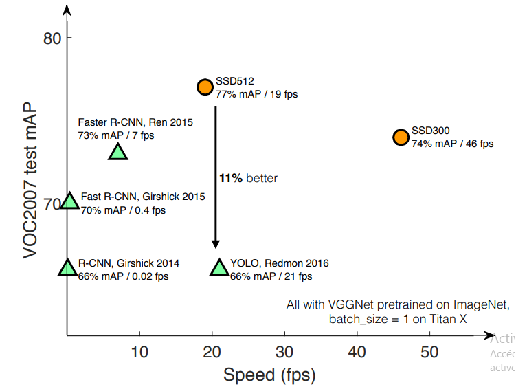
• The following is a scatter plot of speed and accuracy of the major object detection methods (R-CNN, Fast R-CNN, Faster R-CNN, YOLO and SSD300), needless to say that the same model setting (VGG16 as the base network, batch size of 1 and tested on Pascal VOC2007 test set) is used for a fair comparison. Note that YOLO and SSD300 are the only single shot detectors, while the others are two stage detectors based on region proposal approach.

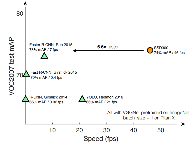
SSD performance comparison (source)

SSD is the only object detector capable of achieving mAP above 70% while being a 46 fps real-time model.

• In terms of accuracy, SSD outperforms YOLO while at the same time being significantly faster with a 25 fps margin.

• Faster R-CNN uses 600x600 input images, SSD achieves comparable accuracy to Faster R-CNN while using lower input size of 300x300. Now it is evident that using larger resolution inputs work better in terms of accuracy, so let’s see how SSD performs with larger inputs with SSD512

SSD performance comparison (source)

Although SSD512 is not a real-time detector like Faster R-CNN, With larger inputs, it performs better than Faster R-CNN with an 80% mAP accuracy.

Further notes

• To further increase real-time speed, consider trying a better base network, since SSD spends 80% of the forward pass on the base network.

• The authors proposed an additional data augmentation step to improve the detection of small-scale objects, referring to it by the “zoom out” operation as opposed to the “zoom in’’ operation mentioned above by random cropping. The technique is to randomly place the standard sized image (e.g. 300x300) onto a canvas up to 16 times larger, then scale it back to the standard size and forward it for training, according to the paper, this added technique improved accuracy by roughly 3% mAP.

Since COCO contains smaller objects than its Pascal VOC counterpart, using the “zoom out” technique when training SSD512 on COCO dataset achieves an accuracy of 80% mAP.

Conclusion

By combining default boxes and multi-scale feature maps in a unified framework, SSD performs faster than state of the art real-time detectors (YOLO) while being as accurate as Faster R-CNN, significantly improving the speed vs accuracy tradeoff.

However, as we stated previously, SSD has its limitations of detecting small objects due to the loss of their semantic features, this drawback is relatively remedied by significant feature implemented in the RetinaNet paper implementing a FPN (Feature Pyramid Network), which uses deep high-level semantic feature maps to construct higher resolution feature layers. The paper presents this concept together with an innovative approach to solving the class imbalance problem.