
Pytorch is an open source deep learning library created in Python that enables tensor operations and automatic differentiation that are crucial to neural network training. Pytorch is one of the leading frameworks and one of the fastest growing platforms in the deep learning research community mainly due to its dynamic computation graph where you can build, change and execute your graph as you go at run time, as opposed to a static graph where you define the graph statically before running it, this restricts the flexibility of the model during training.
Thanks to Pytorch’s dynamic graph you can :
-
Use loops and conditionals in simple python syntax.
-
Easily debug your code using python debugging tools such as pdb or your usual print statements.
-
Use dynamic input variables.
-
Easily build custom structures such as a custom loss function.
Packages
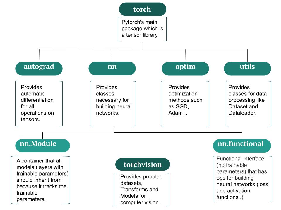
Pytorch packages
Components
1.Tensors
1.1 Tensor creation
A Tensor is a multi-dimensional matrix of data of the same type similar to Numpy arrays, however, we use the former because tensors are moved to the gpu to speed up matrix multiplication resulting in faster training.
Let’s create a simple torch tensor :
import torch

torch.tensor([1,2,3])
Out:
tensor([1, 2, 3])
torch.randn(2,3)
Out:
tensor([[-1.0379,  0.4035,  1.1972],
        [ 0.1631, -0.4870,  0.6018]])
Conversion between torch tensors and numpy arrays is extremely straightforward because they allocate a shared memory space.
import numpy as np

t = torch.eye(3)
# Convert tensor t to numpy array
a = t.numpy()
print('t = {}'.format(t))
print('a = {}'.format(a))
Out:
t = tensor([[1., 0., 0.],
        [0., 1., 0.],
        [0., 0., 1.]])

a = [[1. 0. 0.]
 [0. 1. 0.]
 [0. 0. 1.]]
a = np.array([1,2,3])
# Convert the numpy array a to a tensor
t = torch.from_numpy(a)
print('a = {}'.format(a))
print('t = {}'.format(t))
Out:
a = [1 2 3]

t = tensor([1, 2, 3])
1.2 Tensor attributes
torch.tensor(data=[1,2,3], dtype=torch.float32, device='cpu', requires_grad=False)
Out:
tensor([1., 2., 3.])
-
data(array) : The data of the tensor. -
dtype(torch.dtype) : Type of the elements inside the tensor, if it is saved on the cpu then the dtype istorch.float32, if it is on the gpu the dtype istorch.cuda.FloatTensor. -
device(torch.device) : The device on which the tensor is allocated.
device = torch.device('cuda:0')
torch.tensor([1,2,3], dtype=torch.int32, device=device)
Out:
tensor([1, 2, 3], device='cuda:0', dtype=torch.int32)
requires_grad (bool) : Specifies if the tensor should be apart of the computation graph, if set to False the gradient will not flow back through the graph. Let’s explain this more in depth in the next part.
2. Autograd
After doing a forward pass through the network, you can call .backward() to backpropagate the gradient to the inputs using the chain rule, setting the requires_grad of a Tensor to True allows the gradient to backpropagate through its node in the computation graph, therefore you can access the gradient of this Tensor by calling the .grad method. Theautograd package enables this automatic differentiation.
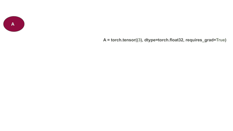
let’s look at an example of this :
A = torch.tensor((3), dtype=torch.float32, requires_grad=True)
A
Out:
tensor(3., requires_grad=True)
B = torch.tensor((2), dtype=torch.float32, requires_grad=True)
B
Out:
tensor(2., requires_grad=True)
C = A * B
C
Out:
tensor(6., grad_fn=<MulBackward0>)
D = torch.tensor((4), dtype=torch.float32, requires_grad=True)
D
Out:
tensor(4., requires_grad=True)
L = C + D
L
Out:
tensor(10., grad_fn=<AddBackward0>)
Compute the gradient of L w.r.t leaf Tensors (i.e Tensors that are not a result of an operation)
L.backward()
The gradient of L w.r.t A
A.grad
Out:
tensor(2.)
The gradient of L w.r.t B
B.grad
Out:
tensor(3.)
The gradient of L w.r.t D
D.grad
Out:
tensor(1.)
For memory saving reason?s you can only access the gradient of leaf Tensors through .grad, BUT you can extract the gradient of intermediate tensors for inspection / debugging by calling .retain_grad() before calling .backward().
Furthermore, by calling .grad_fn you can look at the Function that produced the non-leaf Tensors, of course leaf Tensors will return None as follows.
A.grad_fn
Out:
None
Meanwhile, L is the result of adding two tensors C and D.
L.grad_fn
Out:
<AddBackward0 at 0x7f5dd1093320>
Building the model in Pytorch
Lets build a classifier to recognize images of clothes trained on the MNIST Fashion dataset, the process is as follows:
-
Prepare the data : extract, transform & load the data.
-
Build the network’s architecture.
-
Train the network on training data.
-
Evaluate the model’s performance on testing data.
1. Preparing the data:
import torch
import torch.nn as nn
import torch.nn.functional as F
import torch.optim as optim
from torchvision import datasets, transforms
The Fashion MNIST dataset contains 70,000 samples of 28 * 28 gray scale images, classified into 10 categories (T-shirt/top, Trouser, Pullover, Dress, Coat, Sandal, Shirt, Sneaker, Bag, Ankle boot)
classes = ['T-shirt/top', 'Trouser', 'Pullover', 'Dress', 'Coat',
               'Sandal', 'Shirt', 'Sneaker', 'Bag', 'Ankle boot']
We start by specifying the transformation we want to apply to the images by calling torchvision.transforms, use transform.Compose to apply multiple transformations simultaneously to the input.
transform = transforms.Compose([transforms.ToTensor(),
                                transforms.Normalize((0.5,), (0.5,))])
-
ToTensor: Converts the input image into a torch Tensor. -
Normalize: Normalizes the input image with mean and standard deviation per channel, so for gray scale images we set one value for the mean and one value for the std.
torchvision.datasets class provides popular datasets specific to computer vision, so let’s download the FashionMnist training dataset.
train_dataset = datasets.FashionMNIST(root='./data',
                            train=True,
                            download=True,
                            transform=transform)
Out:
0it [00:00, ?it/s]

Downloading http://fashion-mnist.s3-website.eu-central-1.amazonaws.com/train-images-idx3-ubyte.gz to ./data/FashionMNIST/raw/train-images-idx3-ubyte.gz


26427392it [00:05, 5069325.65it/s]


Extracting ./data/FashionMNIST/raw/train-images-idx3-ubyte.gz


0it [00:00, ?it/s]

Downloading http://fashion-mnist.s3-website.eu-central-1.amazonaws.com/train-labels-idx1-ubyte.gz to ./data/FashionMNIST/raw/train-labels-idx1-ubyte.gz


32768it [00:00, 33503.48it/s]
0it [00:00, ?it/s]

Extracting ./data/FashionMNIST/raw/train-labels-idx1-ubyte.gz
Downloading http://fashion-mnist.s3-website.eu-central-1.amazonaws.com/t10k-images-idx3-ubyte.gz to ./data/FashionMNIST/raw/t10k-images-idx3-ubyte.gz


4423680it [00:03, 1471323.14it/s]
0it [00:00, ?it/s]

Extracting ./data/FashionMNIST/raw/t10k-images-idx3-ubyte.gz
Downloading http://fashion-mnist.s3-website.eu-central-1.amazonaws.com/t10k-labels-idx1-ubyte.gz to ./data/FashionMNIST/raw/t10k-labels-idx1-ubyte.gz


8192it [00:00, 11517.27it/s]

Extracting ./data/FashionMNIST/raw/t10k-labels-idx1-ubyte.gz
Processing...
Done!
-
root(string) : Directory where to save the dataset. -
train(bool) : Set toTrueif the data is used for training, and set toFalseif it’s used for testing. -
download(bool) : Set toTrueto download the dataset in therootdirectory. -
transform(callable) : Set totransformto apply transformations to images, if not set it toNone.
MNIST dataset is already split into 60,000 training samples and 10,000 testing samples, let’s download the testing set.
test_dataset = datasets.FashionMNIST(root='./data',
                           train=False,
                           download=True,
                           transform=transform)
Next, use DataLoader to wrap the dataset into an object for easy access, it also provides batching, shuffling & threading management features.
train_loader = torch.utils.data.DataLoader(dataset=train_dataset,
                                           batch_size=32,
                                           shuffle=True,
                                           )
-
dataset(Dataset): the dataset to load the data from. -
batch_size(int) : the number of samples to pass in a single iteration. -
shuffle(bool) : Shuffle the data for each epoch if set toTrue. -
num_workers(int) : the number of CPU cores/threads used to process a single batch, if set to0the batch will be loaded by the main process, if you use a lot of workers it will increase the memory usage.
We just extracted and loaded our training set let’s do the same for our testing set.
test_loader = torch.utils.data.DataLoader(dataset=test_dataset,
                                          batch_size=32,
                                          shuffle=False,
                                          )
Let’s look at a sample from the training dataset.
Pytorch image tensor is of shape [Channels, Height, Width] and Matplotlib accepts images of shape [Height, Width, Channels], therefore we permute the indices using img.permute(1, 2, 0).
def imshow(img):
    plt.figure(figsize=(10,8))
    plt.imshow(img.permute(1,2,0))
Now, let’s get a training sample from our train_loader.
image, labels = next(iter(train_loader))
imshow(torchvision.utils.make_grid(image,nrow=7))
Out:
Clipping input data to the valid range for imshow with RGB data ([0..1] for floats or [0..255] for integers).
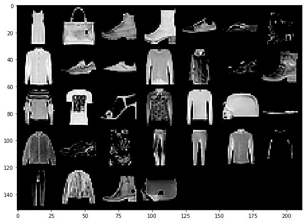
torchvision.utils.make_grid() plots all images in the batch in one grid, even specifying how many images to plot in one row using the nrowargument.
Let’s look at the labels of the first 12 clothe items:
print(list(classes[labels[j]] for j in range(12)))
Out:
['Dress', 'Bag', 'Ankle boot', 'Ankle boot', 'Sneaker', 'Sandal', 'Bag', 'Coat', 'Sneaker', 'Sneaker', 'Pullover', 'Coat']
Because we used thetorchvision.datasets package our dataset was ready to load, this is not the case when you have a custom dataset, so we build an abstract class to represent the dataset, this class should inherit from torch.utils.data.Dataset module.
The class requires a specific methods to be implimented : __len__() to get the length of the dataset and __getitem__() to access a specific data sample by its index, after doing so you can simply load your dataset class into a DataLoader object as we did earlier to benefit from the options mentioned above.
2. Building the network
Pytorch uses OOP to represent the dataset and model, the network class should inherit from nn.Module because it tracks the network’s parameters using .parameters and enables us to easily transfer the model between cpu and gpu using .to(device).
The class has an initialization part and a forward part, the former defines the layers with trainable parameters (e.g: convolution and FC layers) from nn.Module, while the latter defines the structure of those layers from the input along with parameterless layers (e.g: max-pooling and activation functions..) from nn.Functional module.
class Net(nn.Module):

    def __init__(self):
        super(Net, self).__init__()

        # 1 input image channel, 12 output channels, 5x5 convolution kernel, stride of 1 and padding of 2
        self.conv1 = nn.Conv2d(in_channels=1, out_channels=12, kernel_size=5, padding=2, stride=1)
        self.conv2 = nn.Conv2d(in_channels=12, out_channels=20,kernel_size=5, padding=2, stride=1)

        # 7*7*20 input  features, 200 output features
        self.fc1 = nn.Linear(in_features=20*7*7, out_features=200, bias=True)
        self.fc2 = nn.Linear(in_features=200, out_features=10, bias=True)

    def forward(self, x):
        x = F.max_pool2d(F.relu(self.conv1(x)), kernel_size=2, stride=2)
        x = F.max_pool2d(F.relu(self.conv2(x)), kernel_size=2, stride=2)

        # Flatten the 3d tensor to 1d tensor to feed to FC layer
        x = x.view(-1, 20*7*7)
        x = F.relu(self.fc1(x))
        x = self.fc2(x)
        return x
net = Net()
print(net)
Out:
Net(
  (conv1): Conv2d(1, 12, kernel_size=(5, 5), stride=(1, 1), padding=(2, 2))
  (conv2): Conv2d(12, 20, kernel_size=(5, 5), stride=(1, 1), padding=(2, 2))
  (fc1): Linear(in_features=980, out_features=200, bias=True)
  (fc2): Linear(in_features=200, out_features=10, bias=True)
)
We pass the input tensor of size 1x28x28 to the first convolution layer then to a max pooling layer, again to a 2nd convolution layer followed by a 2nd max pooling layer, which outputs a 7x7x20 shape tensor, then the 3 dimensional tensor is flattened to a 1 dim tensor to be fed to the fully connected layers. Eventually the network outputs 10 probability distribution for the 10 classes.
You may be wandering how did we got a 7x7x20 shape output, let’s follow the tensor dimension through the forward pass:
-
Start from the forward method to track the
xinput tensor through the entire structure of layers including layers with non-trainable parameter. -
Decompose the first line of code to inspect the dimension at each layer from the inside out.
-
self.conv1(x) : forwards the 1x28x28 shape tensor
xthrough a convolution layer of 12 filters of 5x5 and padding and stride of 2 and 1 respectively. -
The output width and height dimensions are computed respectively using the following formula:
Where \(w\) and \(h\) are the width and height of the input tensor, \(f\) is the kernel size and \(p\) is the number of padding used.
-
The number of output channels is set in the out_channels attribute, it indicates the number of filters used, the output shape becomes : 12x28x28.
-
F.relu(self.conv1(x)): applying the activation function to a tensor does not alter its shape, it merely introduces non-linearity to learn complex functional mapping between the input and the target. -
F.max_pool2d(F.relu(self.conv1(x)), kernel_size=2, stride=2): applies max pooling of 2x2 filter and stride of 2 to the tensor, following the previous formula the output becomes : 12x14x14.
Using the same procedure through the second line of code, our long-awaited 20x7x7 dimension tensor will be the output.
The x.view() method we used to flatten the tensor specifies the shape to be 2077 number of columns and infers the number of rows by setting the row argument to -1, while maintaining the exact number of tensor elements. We’re going to look at tensor reshaping methods later in this post.
3. Defining the loss and optimizer
Since it is a multi-classification problem, we will use the cross entropy loss.
For the optimizer we will use an Adam optimizer, the parameters of the model stored in ‘ net.parameters()’ along with the learning rate should be provided to the optimizer.
criterion = nn.CrossEntropyLoss()
optimizer = torch.optim.Adam(net.parameters(), lr=0.001)
4. Training the network on training data
Note that before using the optimizer we need to zero out the gradient because in Pytorch the backward() method accumulates the gradient in the backward pass and in order to update the parameters we need the last mini-batch gradient, therefore we zero out the previous gradients before optimizing using optimizer.zero_grad().
epochs = 3

for epoch in range(epochs):
  for i, data in enumerate(train_loader):
      images, labels = data

      # Zero out the gradient
      optimizer.zero_grad()

      # Forward pass
      outputs = net(images)

      # Compute the loss
      loss = criterion(outputs, labels)

      # Backward pass
      loss.backward()

      # Parameter update
      optimizer.step()

      # print the loss value for every 1000 iteration
      if i % 1000 == 0:
              print ('epoch {}/{}, loss:{}'.format(epoch+1, epochs, loss.item()))
Out:
epoch 1/3, loss:2.3015217781066895
epoch 1/3, loss:0.46092498302459717
epoch 2/3, loss:0.37226858735084534
epoch 2/3, loss:0.3666236996650696
epoch 3/3, loss:0.13547854125499725
epoch 3/3, loss:0.18900839984416962
5. Saving and loading the model
The state_dict() object is a dictionary that both Pytorch models and optimizers have to store their parameters, the model.state_dict() maps each of the model layers to their parameters, while optimizer.state_dict() saves the updated parameters and the hyperparameters it uses. This provides excellent flexibility to save, alter and eventually restore your model’s parameters.
# Save the parameters
torch.save(net.state_dict(), PATH)

# Load the parameters
net = Net(*args, **kwargs)

torch.load_state_dict(net.load(PATH))

# Set to testing mode
net.eval()
Dropout and batch norm layers behave differently during training and testing, therefore we set them to training mode using model.train() and to test mode using model.eval(). For this reason, adding ‘ model.eval()’ before inference should be remembered.
6. Evaluating the model on testing data
When evaluating your model you don’t need to compute the gradients and update the parameters, so you should consider using your code inside the context manager with torch.no_grad() to avoid tracking the gradients of the tensors, which reduces memory allocated by the values cached in the forward pass.
correct = 0
total = 0
with torch.no_grad() :
    for images, labels in test_loader:
        images, labels = data
        outputs = net (images)
        # Get the index of high
        _, predicted = outputs.max(dim=1)
        total += labels.size(0)
        #If the prediction matches the provided label
        correct += (predicted == labels).sum()
print('Test Accuracy on testing dataset is : {}%'.format(100 * correct / total))
Out:
Test Accuracy on testing dataset is : 96%
Tensor reshaping methods
The shape of the input tensor changes through the networks layers, therefore the knowledge of tensor reshaping methods gives you greater understanding of what’s going on inside the network and enables you to easily debug your network code.
Here are the tensor reshaping methods:
reshape() : reshapes the tensor while preserving the tensor elements.
t = torch.rand(6,1)
t.reshape(3,2).shape
Out:
torch.Size([3, 2])
squeeze() : removes the axis of dimension 1.
t = torch.rand(1,3)
t.squeeze().shape
Out:
torch.Size([3])
unsqeeze() : adds an axis of dimension 1.
t = torch.rand(3,2)
t.unsqueeze(dim=0).shape
Out:
torch.Size([1, 3, 2])
view() : reshapes the tensor while preserving the tensor elements, just like reshape().
t = torch.rand(3,2)
t.view(-1,6).shape
Out:
torch.Size([1, 6])
flatten() : gets all tensor elements in one dim array to be fed to FC layers.
t = torch.rand(6,2,2)
t.flatten().shape
Out:
torch.Size([24])
PyTorch accepts only mini-batches as input, so it accepts 4-dimensional tensors of shape torch.size([ Batch_size, Num_channels, Hight, Width ]), therefore to pass a single image you should use the above mentioned
unsqueeze()method, it enables you to add an extra dimension of 1 to the batch axis of the tensor shapet.unsqueeze(dim=0).
You can find the full code for this post in the jupyter notebook.
Conclusion
This was an introductory post to Pytorch where we learned about torch packages, tensors and how automatic differentiation works, we also built an effortless classifier that achieved a 96% accuracy on test data. We also learned how to track the input tensor dimension to get deeper understanding of what happens inside the network, making debugging easier.
If you want to learn more about Pytorch, I strongly recommend checking the Pytorch official tutorials for multiple CV, NLP, generative and RL applications. Remember that we learn by doing, so maybe consider running and tinkering with the notebooks in Google Colab.