
Have you tried to implementing QLoRa before? If you are like me and you’re not satisfied with merely skimming the surface, especially with the lack of documentation of the internals of the bitsandbytes library (as of the writing of this post), then this post is for you. While the HuggingFace team explains a bit about FP4 (Float Point 4-bit precision) in their launch post, they do not delve deeply into NF4 (Normal Float 4-bit precision), despite recommending it for better performance.
This gap prompted me to explore the library thoroughly and write the most comprehensive step-by-step breakdown of the bitsandbytes 4-bit quantization with the NormalFloat (NF4) data type to date. This post also intends to be a one stop comprehensive guide covering everything from quantizing large language models to fine-tuning them with LoRa, along with a detailed understanding of the inference phase and decoding strategies.
By the end of this post, you should have a deep understanding of:
- How LLM quantization works and the theory behind LoRa.
- How 4-bit quantization works with the NF4 dtype in detail along with an implementation from scratch of NF4 quantization that returns the exact result as the bitsandbytes implementation.
- Other memory saving techniques that are useful when dealing with limited memory.
- The implementation of QLoRa including injection, finetuning, and final merging with the base model, with a detailed code walkthrough (PEFT code abstracts a lot of things).
- Large language model (LLM) inference process with KV caching.
- Decoding strategies with implementation from scratch.
- Quantization Overview
- GPU Memory Estimation
- LoRa Theory
- Technical Deep Dive into Implementing QLoRa
- 1. Breakdown of 4-Bit Quantization Using NF4 Data Type
- 2. Loading and Configuring the NF4 Quantized Model
- 3. Casting Certain Layers to Full Precision
- 4. Injecting LoRa Trainable Adapters
- 5. Finetuning Process with LoRa
- 6. Strategies for Reducing GPU Memory Usage in LLM Finetuning with STTrainer
- 7. Merging LoRa adapters to base model
- LLM Inference Process
- Decoding Strategies
Quantization Overview
The concept of quantization originates from the field of signal processing, where an information signal is mapped from a continuous input domain to a discrete one. In deep learning, we use quantization to reduce the precision of neural network weights and activations because models are typically over-parameterized, meaning they include a lot of redundancy. This is typically achieved by mapping their values from floating point to a discrete set of integer numbers, e.g, converting them from Float32 into INT8 representation.
A good quantization scheme produces a smaller model size that can simulate the performance of full precision (or half precision) models with minimal loss in accuracy. This leads to a reduced memory footprint as well as a lower I/O memory bandwidth due to less data being transferred, resulting in an overall reduced inference latency. This enables you to run or deploy LLMs on resource constrained devices or even use larger, better performing models. It can be helpful in increasing serving throughput if you have an LLM that is queried by multiple users.
So how is this mapping from floating points to integer values done? This is achieved using linear scaling with a real value factor \(S\) that maps the input range to the output range in the quantized space. This scaling factor \(S\) is simply the ratio of the input range to the output range \(S = \frac{\beta - \alpha}{\beta\_{\text{quant}} - \alpha\_{\text{quant}}}\). The result is offsetted with an integer zero-point \(Z\) value that maps zero in float range to its corresponding zero value in the integer range.
There are two types of quantization symmetric and asymmetric quantization, each computing the quantization parameters \(Z\) and \(S\) differently. We describe below the two approaches to quantizing real values to a signed b-width bit integer representation. Symmetric quantization creates a quantized space that is symmetric around 0, where the value 0.0 in the float space is mapped exactly to 0 in the integer space. In contrast, asymmetric quantization maps 0.0 to a specific quantized zero-point \(Z\). The goal of specifying this point is to ensure that 0.0 in the input data is quantized without error, this can be useful in neural network operations that contain zeros, where we want a consistent result, an example of this would be zero padding.
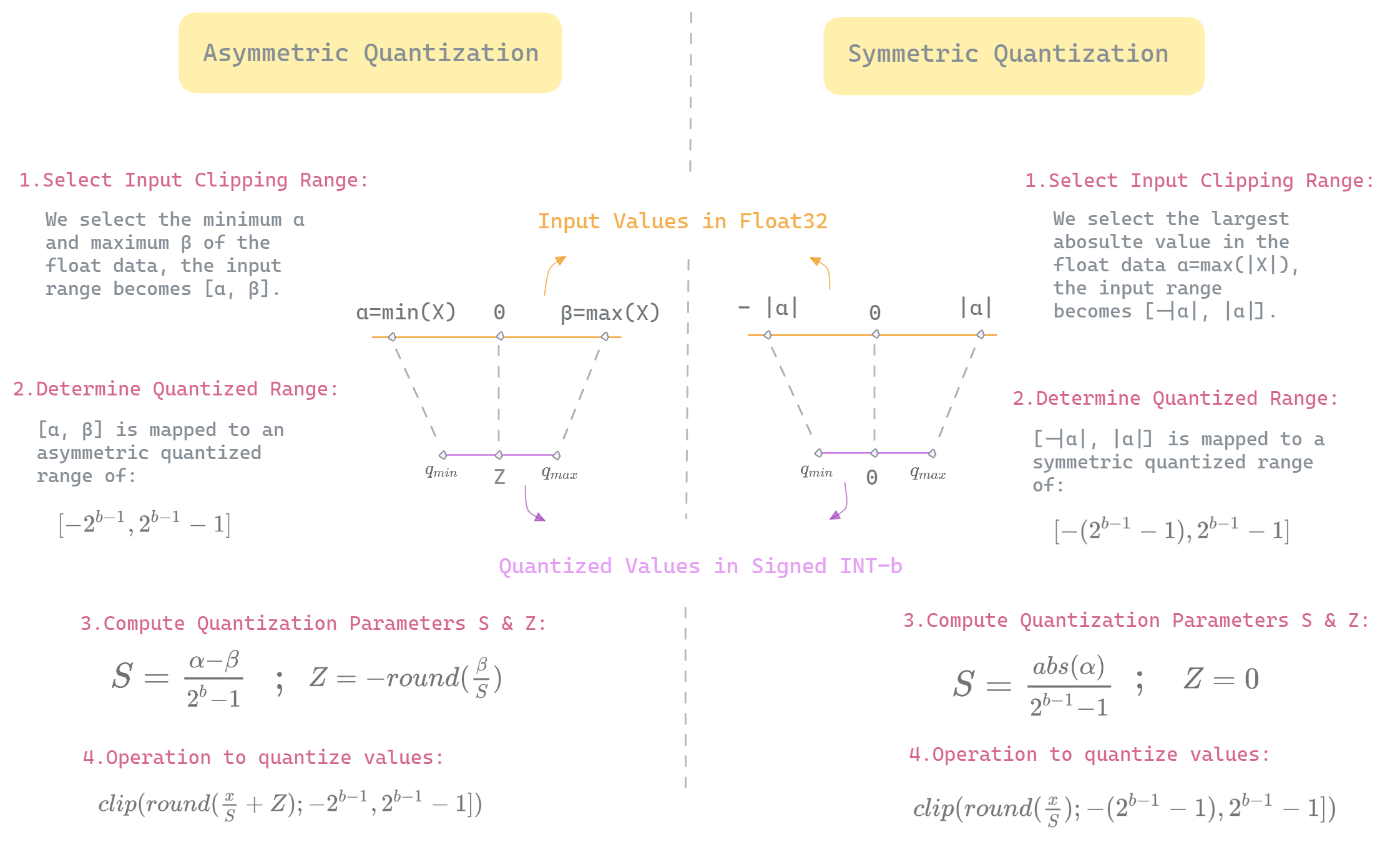
Illustration detailing both symmetric and asymmetric quantization approaches to quantizing floating-point values in 32 bits to a signed integer in b-width bits — Created by Author.
The quantization process in both approaches start by determining the clipping range values, an operation often referred to as calibration. The clipping range in symmetric mode \([α , −α]\) is symmetric with respect to zero, while the clipping range \([α, β]\) in asymmetric quantization is, unsurprisingly, asymmetric around zero, that is \(−α ≠ β\). Next we use the clipping range values to compute the quantization parameters \(S\) and \(Z\). Afterward, we scale down the input data using \(S\) (also offsetting with \(Z\) in asymmetric mode) and round the result to the nearest integer. If the produced value falls outside the limits of the quantized domain, we use the clip operation to restrict it within the specified bounds.
The dequantization process approximates the original floating point values from the quantized integer values by simply reversing the quantization operation. This is expressed as \(x = S*x_q\) in symmetric mode and \(x = S(x_q-Z)\) in asymmetric mode. Dequantization can be used for different reasons, for instance, dequantizing some output that must be fed to an operation requiring greater precision input to ensure better numerical stability or simply dequantizing the output of a network.
It’s important to note that dequantization doesn’t accuratly reconstruct the original float data, due to the quantization error that is introduced by to the rounding and clipping operations in the quantization process. Therefore, the best quantization approach is the one that minimizes this error and effectively reduces information loss associated with reducing precision.
With two quantization schemes, the question arises, when should each approach be used?
Choosing between symmetric and asymmetric quantization
It depends mainly on the distribution of the data that we want to quantize. If the original data is normally distributed, symmetric quantization is preferred, whereas asymmetric quantization is more suitable for skewed data.
It’s important to note that asymmetric quantization is far more complicated than symmetric quantization to implement, as the former includes the additional \(Z\) term, which during matrix multiplication, introduces computational overhead leading to increased latency. This pleads the question, if this is the case, why not simply apply symmetric quantizaton on skewed data? Let’s explore this by considering an example with one of most common operations in neural network that systematically generates skewed data, the ReLU activation function.
Before delving into the case study, it’s important to point out that the representational capacity of a \(k\)-bit width refers to the number of distinct values that can be represented with \(k\)-bit width, which is \(2^k\) possible unique values. For instance, 8-bit quantization allows for 256 discrete values, while 4-bit quantization allows for 16 values. This can be effectively represented with a histogram with each bin representing a single possible value.
In our case study, I use symmetric quantization to reduce the precision of the Relu output from float32 to int8, meaning, this representation allows for 256 discrete bins ranging from -127 to 127 values:
X = torch.randn(200, dtype=torch.float32)
X = F.relu(X)

bit_width = 8
alpha = torch.max(X)

# determine clipping range
r_max = 2 ** (bit_width - 1) - 1
r_min = -(2 ** (bit_width - 1) - 1)

# compute scaling factor S
scale = alpha / r_max

# symmetric quantization operation
quantized_data = X/scale
quantized_data = torch.clamp(torch.round(quantized_data), min=r_min, max=r_max).to(torch.int8)

plot_histogram(quantized_data, bit_width, quantized_data)
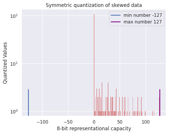
Using symmetric quantization to convert the Relu output from float32 to int8 values, we select the largest absolute value in the data α, and create a clipping range of [ -α , α], then scale the values down to map them to a quantized domain of [-127, 127]. This representation allows for 256 discrete bins ranging from -127 to 127 values. These quantized limits are depicted in the histogram by the blue and purple vertical lines. Link to code for converting to 8-bit via symmetric quantization and histogram plotting — Created by Author.
We can clearly see in the histogram that half of the bins to the left of zero are not utilized at all, this leads to a more limited data representation, where instead of utilizing the entire 256 values assumed in an 8-bit representation, it only uses half of that, which is 128 values. This is equivalent to using a 7-bit format (\(2^7=128\)) resulting in one bit that is completely wasted out of the 8 bits.
However, if we use asymmetric quantization on Relu output, the full range of quantized values will be fully utilized, because the clipping range becomes \([r_{min}=min(X),r_{max}=max(X)]\) instead of \([ -α= - max(∣X∣) , α=max(∣X∣)]\) which includes the values that actually show up in the input data.
To conclude, applying symmetric quantization to skewed data might allocate a significant portion of the quantized range to values that are unlikely to occur in practice, which makes asymmetric quantization more suitable for this type of data.
Some background on non-uniform quantization
Now that you’ve reached this part of the post, I should point out to you that all of the previously mentioned information about quantization relates to linear quantization, otherwise reffered to as uniform quantization, which involves linear scaling with \(S\) and results in equally spaced quantized values with a constant step size.
The constraint of using equally spaced quantized values in uniform quantization is that it creates a representation that may not approximate the distribution of the input data well, increasing the performance gap between the full precision and its quantized counterpart.
That’s why non-uniform quantization also exists. Non-uniform quantization uses a non-linear function which generates values that are not necesseraly equally spaced, i.e, it can use non-constant steps resulting in different quantized levels.
As such, non-uniform quantization with the same number of bits can create a representation that is more flexible to approximate the distribution of full precision values better, thus reducing the quantization error and leading to a better performance compared to uniform quantization.
For instance, neural network weights typically follow a Gaussian distribution with most of the values clustered around 0. In this case, applying non-uniform quantization will better represent the distribution of the weights. For example, we can use a non-uniform quantization method with increased resolution or smaller step sizes around 0.
However, the challenge with non-uniform quantization is that using non-linear function involves look-up tables and additional logic that is not hardware efficient. Although a lot of recent work has been proposed to address this issue, one example is Power-Of-Two quantization, which uses a base-2 logarithmic to quantize the numbers into powers of 2, allowing the dot-product to be accomplished using bit shifting instead of multiplication, which is more hardware friendly.
Consequently, uniform (linear) quantization is still considered the standard in most libraries that provide quantization support like Nvidia’s TensorRT-LLM, HuggingFace’s Quanto and PyTorch’s built-in quantization module, mainly due to its simpler implementation.
GPU Memory Estimation
Finetuning large models or simply running inference requires substantial GPU memory because it requires the model weights and intermediate computations to be loaded into the GPU’s memory.
This memory bottleneck is fundamentally imposed by the von Neumann architecture in current computing systems, where the main system memory is separated from the compute processing units on GPU. Therefore, all data required for neural network computations must be transferred from main memory to GPU memory (VRAM). This data in question includes the model weights, the gradients, the activations and optimizer states, all need to fit into the GPU memory.
Furthermore, the bottleneck is due to memory hierarchy, where memory component in computing systems can be arranged hierarchically in terms of storage, speed and cost. With the main memory being relatively cheap yet offering larger storage with slower access to data, while GPU memory being expensive with smaller storage but offering faster access speeds.
To give you an idea of how much GPU memory is required for finetuning, a 7 billion parameter model loaded in 16-bit precision format, means each parameter is represented by 2 bytes of memory, thus you need 14 GB of GPU memory just to load the model weights alone. For a 32-bit precision, where each parameter is represented by 4 bytes, you would need 28 GB of GPU memory. Additionally, you have to account for some memory overhead, typically extra GBs to store forward activations, gradients and optimization states.
Memory requirement can be estimated using the following formula :
\[VRAM\_requirement = total\_number\_of\_parameters\ * \ number\_of\_bytes\_per\_parameter\]LoRa Theory
As we mentioned above, finetuning language models is computationally expensive, almost prohibitive when dealing with LLMs that contain parameters in the order of tens of billions or more. As a result, many memory-efficient finetuning methods have been developed, one of which is LoRa (Low-Rank Adaptation of Large Language Models) which is introduced as a parameter-efficient finetuning approach that enables finetuning large models on resource-constrained devices, making it possible to adapt powerful language models to downstream tasks for everyone.
The LoRa paper states the following “LoRa expresses the weight updates ∆W as a low-rank decomposition of the weight matrix”. Let’s break this down to fully understand what does this mean. First, let’s understand the terms, mathematically, the rank of a matrix refers to the number of linearly independent vectors in a matrix. Linearly independent vectors are vectors that can not be produced by linearly combining other vectors. As a result, they are considered the most important ones in the matrix that can not be constructed from others vectors and contain unique information. With this in mind, for an \(m\) x \(n\) matrix \(A\), if the rank of this matrix is less than the number of its columns or rows, \(rank (A) < min(m, n)\), we say that A is rank-deficient or has a low-rank.
The Low-Rank Adaptation paper is influenced by ideas in the Li et al. and Aghajanyan et al. papers that show that language models are over-parameterized and have a very low intrinsic dimension that can be effectively represented using fewer dimensions.
It turns out that LLMs have a low dimension rank structure, meaning that important features and patterns in the model can be represented using significantly fewer dimensions, efficitively reducing the model complexity.
Based on these findings, the authors hypothesized that the finetuned part \(ΔW\), which is the change in weights during model adaptation — where the weights are adapted to the new task — also has a low intrinsic rank. The change in the weights \(ΔW\) refer to the the difference between the finetuned parameters \(W_{finetuned}\) and the pre-finetuned parameters \(W_{pretrained}\) in a single layer.
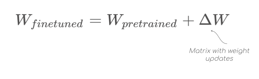
\(∆W\) having a low rank implies that it can be decomposed into two smaller matrices \(A\) and \(B\) (hence low-rank decomposition) which are then adapted to the new dataset.
Instead of learning the highly dimensional weight update matrix \(ΔW\) like in regular full finetuning, LoRa approximates \(ΔW\) with the product of two significantly smaller matrices and learn their parameters instead.
To examine this closely, a \(d\) x \(k\) matrix \(ΔW\) can be factored as \(ΔW=BA\), where \(A\) is a \(d\) x \(r\) matrix and \(B\) is a \(r\) x \(k\) matrix, where \(r\) denotes the LoRa rank with \(r << min(d, k)\). Using this approach, the total number of parameters becomes \(r(d+k)\) instead of \(d\) x \(k\).
For instance, using a linear layer with a \(1000\) x \(1000\) weight matrix and a rank value of \(r=3\), with LoRa, the number of trainable parameters for this layer would be reduced from \(1,000,000\) to \(6,000\). This is effectively reducing \(99.4\)% of the parameters in a single layer!
Note that LoRa rank r is a hyperparameter that determines the shape of the A and B matrices and evidently, selecting a smaller r value results in far fewer parameters to learn during finetuning, however it might not capture all the knowledge in the new dataset.
Now that we understand that LoRa replaces the weight update matrix \(ΔW\) of selected layers with much smaller matrices A and B, how are these matrices created?
Initially, the paper mentions that the parameters of matrix \(A\) are initialized from a random Gaussian distribution while the parameters of matrix \(B\) are initialized with zeros, this means that \(BA\) is equal to zero intially before being updated during finetuning.
Furthermore, \(ΔW\) is scaled by the factor of \(\dfrac{α}{r}\) , where \(r\) is the rank and \(α\) is a hyperparameter needed for scaling.
The objective of this scaling is to reduce the risk of adapters overfitting the data when using higher rank value and to maintain a consistent learning behavior for different rank values.
Here is a pseudocode example, but for a detailed description of the implementation please refer to this section.
class LoRaAdapter(nn.Module):
    def __init__(self, rank, alpha, d, k):
        super().__init__()
        self.scale_factor = alpha/rank
        # assuming weight matrix is of (d x k) dimensions
        self.A_matrix = nn.Parameter(torch.randn(d, rank))
        self.B_matrix = nn.Parameter(torch.zeros(rank, k))

    def forward(self, x, W_0):
        W_0.requires_grad = False
        result = W_0 @ x + ((self.A_matrix @ self.B_matrix) @ x) * self.scale_factor
        return result
Only \(A\) and \(B\) are updated, this implies that the gradients and the parameter updates in the backward pass are computed only for A and B, while keeping the original weight matrix \(W_0\) (the 4-bit quantized layer) frozen. This results in a significant reduction in memory space used to store the checkpoints during finetuning. As such, you’ll find that LoRA produces checkpoints of about few MB, unlike the memory intensive full finetuning that typically causes OOM errors. Furthermore, LoRa leads to a substantial reduction in computational costs and massive speed-up in the fine-tuning process since it focuses on a smaller set of parameters instead of updating the billion parameters in the LLM, all while producing a model with a comparable performance to full finetuning.
Don’t take my word for it, here is the empirical results from the paper:
The paper uses GPT-3 175B LLM as an example. Using LoRa finetuning, the number of trainable parameters was reduced by 10,000 times compared to full finetuning. Additionally, VRAM consumption during finetuning decreased from 1.2TB to 350GB, while checkpoint size was downsized from 350GB to 35MB. This translated into a 25% speedup on the finetuning process.
What’s unique about LoRa is that it doesn’t have any inference latency cost. After finetuning, the adapted weight matrices are simply combined with the original weight matrices, as you will see in this section. This is exceptionally useful when switching between tasks. That is, you can use the same base model finetuned on different downstream tasks and simply swap LoRa adapters for different tasks, as opposed to reloading multiple large models with the same large size, which is ofcourse memory and time inefficient.
Using LoRa, task switching becomes more efficient because it consists of loading the weights of the base model one time and simply swapping the LoRa adapters for different tasks with minimal overhead instead of loading multiple finetuned models with the same large size.
Although LoRa adapters can be injected into any linear layer in the LLM architecture, in the paper, it exclusively injects the adapters into each of the projection matrices in the self-attention module, which are \(W_{query}\), \(W_{key}\), \(W_{value}\), and \(W_{output}\).
You’ll gain a deeper understanding of LoRa in this section (part 4, 5, 7).
Technical Deep Dive into Implementing QLoRa
Now that we have a solid theoritical understanding of how the LoRa finetuning approach works and some background on quantization, we can delve into how QLoRa combines the two concepts to dramatically reduce GPU memory usage when finetuning large models.
This section aims to be a technical deep dive into implementing QLoRa. Libraries involved in applying QLoRa:
- 4-bit quantization is implemented in the bitsandbytes quantization library created by Tim Dettmers which also offers 8-bit quantization among other techniques like 8-bit optimizers.
- HuggingFace 🤗 team provides LoRa finetuning via
PEFTlibrary (which provides several parameter-efficient finetuning methods) which is integrated with the Transformers library. - The HuggingFace 🤗 team have integrated bitsandbytes with the 🤗 ecosystem, to enable finetuning methods available in
PEFTto be applied on quantized (4-bit or 8-bit) base models with very few lines of code.
1. Breakdown of 4-Bit Quantization Using NF4 Data Type
bitsandbytes provides 4-bit quantization using block-wise k-bit quantization, this is applied to the model’s linear layers through the Linear4bit class, which converts linear modules from nn.Linear to bnb.nn.Linear4Bit layers.
Let’s walk through the steps that a weight matrix \(W\) goes through to be converted to the NF4 data type using block-wise quantization:
1. Flatten the weight matrix \(W\) into a one-dimensional sequence.
2. Then split \(W\) into equal sized blocks.
3. Normalize each block with its absolute maximum value to make sure the weights fit within the quantization range of [-1, 1] — This is the scaling operation where the scaling factor S is the absolute maximum value, as a result the scaling factor of each block is stored for the dequantization process as a tensor with a length equal to the number of blocks.
4. The actual quantization mapping uses a set of predefined unique 16 float values [\(q_1, . . . , q_{16}\)] suggested by the paper to map each value normalized value \(x_i\) in the block to the nearest quantized value \(q_i\) in the set. These NF4_quant_levels are further referenced in both the paper (in Appendix E) and the code.
NF4_quant_levels = [-1.0, -0.6961928009986877, -0.5250730514526367, -0.39491748809814453, -0.28444138169288635, -0.18477343022823334, -0.09105003625154495, 0.0, 0.07958029955625534, 0.16093020141124725, 0.24611230194568634, 0.33791524171829224, 0.44070982933044434, 0.5626170039176941, 0.7229568362236023, 1.0]
So why these NF4_levels values in particular?The NF4 data type introduced in the QLoRa paper uses 4-bit quantile quantization to generate a set of quantization levels which are then normalized to fit a range of [-1, 1]. This NF4 levels representation is best suited for normally distributed data with high precision around zero, which is the case for neural network weights which mostly follow Gaussian distribution, hence the name “Normal Float”.
k-bit quantile quantization estimates \(2^b\) equally spaced quantile values \(q_i\) where \(b\) is the desired bit-width for quantization. These estimated quantiles represent the quantization levels based on the quantiles of the normal distribution. To achieve this, the bitsandbites library uses the quantile function — also referred to as the inverse cumulative distribution function (ICDF) — implemented using scipy.stats.norm.ppf to generate these values. These quantiles are then normalized by the maximum value to achieve a range of [-1, 1]. Furthermore, Qlora uses asymmetric quantization to quantize \(0\) in the input tensor to a constant non-zero value Z. This results in exactly \(2^{b-1} + 1\) positive values and \(2^{b-1}\) negative values in the representation (this makes it 9 positive values and 8 negative values in NF4_quant_levels).
Now that we know from where these value come from, the bitsandbites library uses midpoints between NF4 values as bins and compares each input value \(x_i\) to determine which bin the input value \(x_i\) falls into. It then assigns \(x_i\) to the closest \(q_i\) that falls within the bin.
TL;DR : NF4 uses a mapping table of 16 levels
NF4_quant_levelsto map each input value to the nearest NF4 value. These are quantiles of a theoritical normal distribution that are normalized to fit a range of [-1, 1] to make them compact around 0. This means, the NF4 quantization is an asymmetric, non-uniform quantization scheme that is applied independently to each block of the input weights . These produced floating points quantization levels are ideal for normally distributed data like neural network weights with high precision around zero.
The following steps 5 and 6 contain additional logic to store the final quantized values:
5. Each quantization level is represented with a 4 bits binary value as referenced in this part of the code. These are the binary representation of unsigned 4-bit integers format uint4, we will see at end of step 6 why we use the uint4 representation. For instance, this function uses these binary values to map back to the quantization levels during the dequantization process.
NF4_quant_4bit = [0b0000, 0b0001, 0b0010, 0b0011, 0b0100, 0b0101, 0b0110, 0b0111, 0b1000, 0b1001, 0b1010, 0b1011, 0b1100, 0b1101, 0b1110, 0b1111]
# decimal representation of the above uint4 binary values:
NF4_quant_4bit = [ 0,  1,  2,  3,  4,  5,  6,  7,  8,  9, 10, 11, 12, 13, 14, 15]
6. Finally, pack the quantized 4-bit tensor into torch.uint8 dtype (an 8-bit unsigned integer representation).
Explaining both the reasoning and logic behind compacting 4-Bit values into 8-Bit formats
Admittedly, this part intially threw me off, as I was expecting the 4-bit representation to be packed into a 4-bit data type which assumes exactly 16 unique values, not an 8-bit data type with 256 unique values. However, after going through the code, it turns out the author of bitsandbytes converts the 4-bit values into 8-bit by packing two 4 bit values into a single 8-bit value, this results ofcourse, in a different shape for the quantized tensor. This is because PyTorch does not support 4-bit data types and the smallest type it supports is 8-bits — as of the writing of this post
Furthermore, the reason it uses an 8-bit integer format and not an 8-bit floating point format
FP8is due to the lack of native support forFP8in PyTorch. The packing operation is exactly what Pytorch’s new data type ‘quantized 4-bit integer’torch.quint4x2does as well, as you can see in the documentation. The packing of the two 4-bits values to 8 bits is very straightforward using simple bitwise operations. The actual packing step in bitsandbytes is performed in this part of the code, but make sure to follow along to see our implementation.
To make sure my understanding of the 4-bits quantization with the NF4 data type (described in the above steps) is accurate, I implemented it from scratch on a small dummy input (first code snippet) and compared it to the bitsandbytes implementation (second code). Thankfully, the produced values are exactly equal.
Note that the smallest block size used in bitsandbytes is 64 elements and since my input \(W\) has 20 elements, bitsandbytes will treat this tensor as a single block and no splitting will be involved, as a result I didn’t implement it in below.
import torch

NF4_quant_levels = torch.tensor([-1.0, -0.6961928009986877, -0.5250730514526367, -0.39491748809814453, -0.28444138169288635, -0.18477343022823334, -0.09105003625154495, 0.0, 0.07958029955625534, 0.16093020141124725, 0.24611230194568634, 0.33791524171829224, 0.44070982933044434, 0.5626170039176941, 0.7229568362236023, 1.0])

#  binary representation of uint4 values (used 4-bit binaries instead of decimals for illustration purposes)
nf4_quant_4bit = torch.tensor([0b0000, 0b0001, 0b0010, 0b0011, 0b0100, 0b0101, 0b0110, 0b0111, 0b1000, 0b1001, 0b1010, 0b1011, 0b1100, 0b1101, 0b1110, 0b1111])

# generated tensor of [5, 4] shape
W = torch.tensor([[ 0.4767, -0.2921,  0.0787, -0.1018],
                  [-0.3453,  0.3834, -0.0107, -0.4692],
                  [-0.4072, -0.2996, -0.4942, -0.2640],
                  [ 0.0125,  0.2962,  0.3123, -0.4705],
                  [-0.1982, -0.1545,  0.3358, -0.4086]])

flat_W = W.flatten()

# normalize the tensor using absmax to fit within [-1, 1]
max_val = flat_W.abs().max()
normalized_W = flat_W / max_val

# map each input value to its nearest quantization level - then to its 4-bit binary representation
quantized_W_4bits = torch.zeros(normalized_W.shape, dtype=torch.int)
for i, val in enumerate(normalized_W):
    closest_level = torch.argmin(torch.abs(NF4_quant_levels - val)) # get the index of closest quantization level
    quantized_W_4bits[i] = nf4_quant_4bit[closest_level]

print(quantized_W_4bits)
# Output: [15,  2,  9,  5,  1, 14,  7,  0,  1,  2,  0,  2,  7, 13, 13,  0,  3,  4, 14,  1]

packed_W_8bits = []
for i in range(0, len(quantized_W_4bits), 2):
    # Courtesy of https://www.geeksforgeeks.org/store-two-numbers-in-one-byte-using-bit-manipulation/
    # take each pair of 4-bit values in quantized_W_4bits and combine them into packed_W_8bits by shifting
    # the first 4 bits to the left using the left shift operator '<<' and combining them using the OR | operation
    result = (quantized_W_4bits[i] << 4) & 0xff
    result =  result | quantized_W_4bits[i + 1]
    packed_W_8bits.append(result)

# set it as torch.uint8
packed_W_8bits = torch.tensor(packed_W_8bits, dtype=torch.uint8)

print(packed_W_8bits)
# Output: tensor([242, 149,  30, 112,  18,   2, 125, 208,  52, 225], dtype=torch.uint8)
To demonstrate how packing the first pair of quantized_W_4bits, which are (15, 2) results in 242 in packed_W_8bits:
we represent 15 in binary as 1111 , while 2 is is represented as 0010. Following the two operations bitwise operations as follow (1111 << 4) | 0010 = 11110000 | 0010 = 11110010 ; the result 8 bit number 11110010 is equal 242 in decimal format.
Here is a bitsandbytes code you can run if you want to check the output of 4-bit quantization with NF4 dtype yourself — it results in the same output.
import bitsandbytes as bnb
from bitsandbytes.nn import Linear4bit, Linear8bitLt
import torch

W = torch.tensor([[ 0.4767, -0.2921,  0.0787, -0.1018],
                  [-0.3453,  0.3834, -0.0107, -0.4692],
                  [-0.4072, -0.2996, -0.4942, -0.2640],
                  [ 0.0125,  0.2962,  0.3123, -0.4705],
                  [-0.1982, -0.1545,  0.3358, -0.4086]])

print(W.weight.dtype)
# Output: torch.float32

# 4-bit quantization with NF4 datatype
quantized_W = bnb.nn.Linear4bit(
    W.in_features,
    W.out_features,
    bias=False,
    quant_type="nf4",
    device="cuda")

quantized_W.weight = bnb.nn.Params4bit(data=W.weight, requires_grad=False).to("cuda")

print(quantized_W.weight.dtype)
# Output: torch.uint8

print(next(quantized_W.parameters()).flatten())
# Output: tensor([242, 149,  30, 112,  18,   2, 125, 208,  52, 225], dtype=torch.uint8)
Moreover, the reason bitsandbytes uses an unsigned uint8 for packing instead of signed integers int8 is that int8 can represent negative values by reserving the bit furthest to the left as the sign bit. However, during the packing step, the left shifting operation can become tricky when dealing with the sign bit. Using uint8 removes this complexity, by keeping only the bits of the actual two 4-bit numbers without including the sign bit. That is why, in step 5 it uses the uint4 format (ranging from 0 to 15) and not int4 (ranging form -8 to 7) to represent each quatized 4-bit value.
TL;DR : In step 6, it’s compacting two
uint4numbers into a singleuint8number. This implementation effictively reduces the model memory footprint to half of 8-bit format. Memory wise, this is equivalent to using a 4-bit quantization format. This is the current Pytorch implementation of any sub-8 quantization. For instance, in 2-bit quantization (given an efficient quantization mapping scheme with minimal quantization error) each value is mapped into a 2-bit value, then each four 2-bit values are packed into a single 8 bit value, achieving the same memory efficiency as a 2-bit quantization would.
2. Loading and Configuring the NF4 Quantized Model
In this section, I explain the configuration choices necessary for implementing of 4-bit quantizated model, this is followed by a step by step process for implementing LoRa finetuning using this quantized model.
Up to this point, we have a model whose linear layers are quantized as NormalFloat 4-bit data type (NF4) and converted from
nn.Lineartobnb.nn.Linear4Bit. Thanks to the integration of the two libraries (bitsandbytes and 🤗’sTransformers) it only takes one step to load the model and quantize it, by enablingload_in_4bitflag and settingbnb_4bit_quant_typeto NF4 usingBitsAndBytesConfigfromTransformeras follows.
from transformers import BitsAndBytesConfig

nf4_config = BitsAndBytesConfig(
   load_in_4bit=True,
   bnb_4bit_quant_type="nf4",
   bnb_4bit_compute_dtype=torch.bfloat16,
   bnb_4bit_use_double_quant=True)


base_NF4_model = AutoModelForCausalLM.from_pretrained("openlm-research/open_llama_3b", quantization_config=nf4_config)
print(base_NF4_model.is_loaded_in_4bit)
# Output: True
What does bnb_4bit_compute_dtype do?
We can specify the data type to use for computation via the bnb_4bit_compute_dtype argument. This determines the desired target dtype for the dequantization process (regardless of the dtype used for the input), you’ll see its use in this section.
Furthermore, you can set bnb_4bit_compute_dtype to float32 (the default) or bfloat16 (16-bit BrainFloat), if you’re not familiar with with bfloat16, this is a great opportunity to learn about it as it’s commonly used in deep learning. Here is what you need to know:
16-bit BrainFloat is a floating point representation developed by Google Brain tailored for deep learning models. This representation has the same number of bits as
float16but with a different allocation of bits, assigning 8 bits for the exponent as opposed to 5 bits infloat16. The increased exponent width offers a larger dynamic range, meaning it can represent a larger range of values (dynamic range is the ratio of the largest to smallest positive value). As a result,bfloat16has a comparable performance asfloat32with half the number of bits. This offers more flexibility to represent smaller and larger values in the network, reducing numerical underflows and overflows all while using less memory during training.
Therefore, it’s recommended to use bfloat16 as bnb_4bit_compute_dtype to perform operations. Consequently, the weights will be dequantized from 4-bits in NF4 to 16-bits in bfloat16 dtype.
What does bnb_4bit_use_double_quant do?
At the normalization step of block-wise quantization, we mentioned that the scaling factors, which are the absolute maximum values, are stored for dequantization. These scaling factors are essentially quantization constants that require additional space to be stored. To address this, the QLoRa paper suggests a solution to further reduce memory storage, which is to quantize the quantization constants themselves using block-wise quantization. This way, we end up with both quantized weights and their corresponding quantization constants being quantized as well. This is referred to as double or nested quantization. According to the paper, double Quantization saves an average of about 0.37 bits per parameter, approximately 3 GB for a 65B model.
3. Casting Certain Layers to Full Precision
After loading the quantized base model, it’s recommended to run the following line of code:
base_NF4_model = prepare_model_for_kbit_training(base_NF4_model)
What does it actually do?
After quantizing all of the linear layers in the model, it’s important to cast some layers back to float32 (fp32) for a better numerical stability. This function casts some layers to float32, specifically, it upcast all normalization layer (BatchNormalization or LayerNormalization) to fp32 because they contain reduction operations like sum and average, which can cause NaN loss values when performed with reduced precision. Therefore, to maintain as much information as possible, we use higher number of bits.
In addition to normalization layers, the function also upcasts the embedding and LM head layers. Furthermore, it freezes the entire model and enables gradient checkpointing, which we will discuss later in the post.
Inspecting the model before calling prepare_model_for_kbit_training :
# normalization - embedding - LM head layers
print(base_NF4_model.model.norm.weight.dtype, base_NF4_model.lm_head.weight.dtype, base_NF4_model.model.embed_tokens.weight.dtype)
# Output : (torch.float16, torch.float16, torch.float16)

print(base_NF4_model.is_gradient_checkpointing)
# Output : False
After calling prepare_model_for_kbit_training :
print(base_NF4_model.model.norm.weight.dtype, base_NF4_model.lm_head.weight.dtype, base_NF4_model.model.embed_tokens.weight.dtype)
# Output : (torch.float32, torch.float32, torch.float32)

print(base_NF4_model.is_gradient_checkpointing)
# Output : True
4. Injecting LoRa Trainable Adapters
Next, we setup LoraConfig, where we specify the layers to inject the loRa adapters into, using target_module. Alternatively you can select all linear layers instead of just few by setting target_modules="all-linear". Following my example I specify the attention and MLP modules in target_modules.
This is also where we define the rank dimension, which determines the shape of the adapter matrices, as well as the Lora dropout, which we mention its use at this section.
target_modules =  ['down_proj', 'gate_proj', 'k_proj', 'o_proj', 'q_proj', 'up_proj', 'v_proj']

lora_config = LoraConfig(
    r=8,
    lora_alpha=16,
    target_modules="all-linear",
    lora_dropout=0.1,
    task_type="CAUSAL_LM",
    bias="none")
Next, we wrap the configuration lora_config with get_peft_model to create a trainable PeftModel :
peft_model = get_peft_model(base_NF4_model, lora_config)
But what does this line of code actullay do ?
-
It creates the adapters, we’ve mentioned earlier that
LoRa_Ais initialized from a Gaussian distribution, however the PEFT library initializes the matrix from Kaiming-uniform distribution while initializing theLoRa_Bmatrix with zeros. -
It then injects these matrices into the layers defined in
target_modules. -
It makes these adapter weights trainable while keeping the rest of the quantized model frozen.
5. Finetuning Process with LoRa
How are the forward & backward phases performed with LoRa adapters?
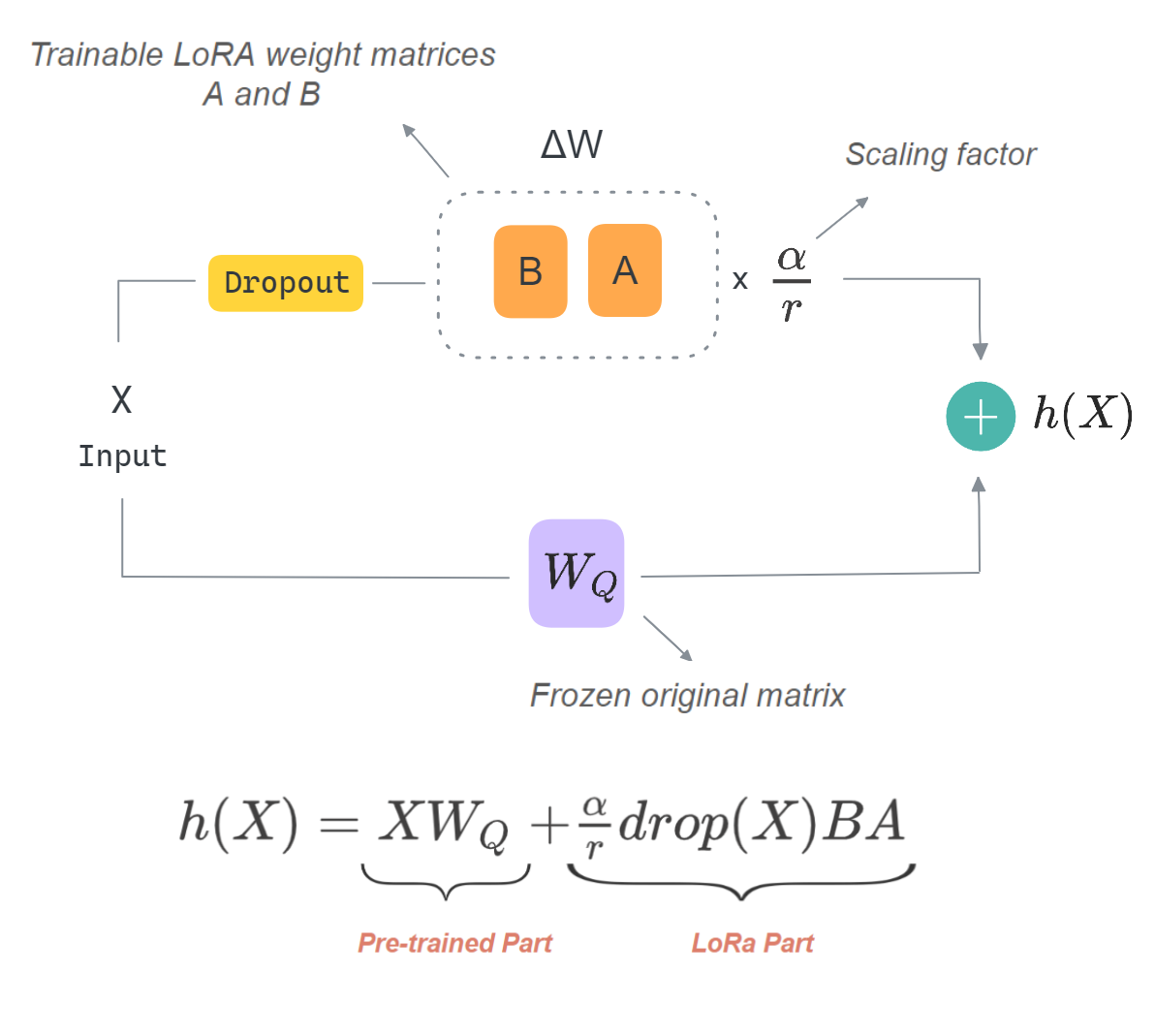
Illustration showing part of forward pass of input X in layer \(W_Q\) which we selected to inject loRa adapters into (layer specified in target_modules). This implementation is specific to the QLoRa paper, not the LoRa paper — Illustration Created by Author.
- As you can see above, the trainable weight matrices \(A\) and \(B\) (which constitute \(ΔW\)) are simply injected into the existing model layer \(W_Q\), as opposed to another existing solution that also uses adapters but adds them as separate layers sequentially to the Transformer architecture, introducing additional inference latency. The layer weight itself \(W_Q\) is kept frozen.
- LoRa dropout introduced in the QloRa paper and is applied to the input \(X\) before multiplying by the matrices \(A\) and \(B\). You can set the value of the
lora_dropouthyperparameter inLoRa_config.
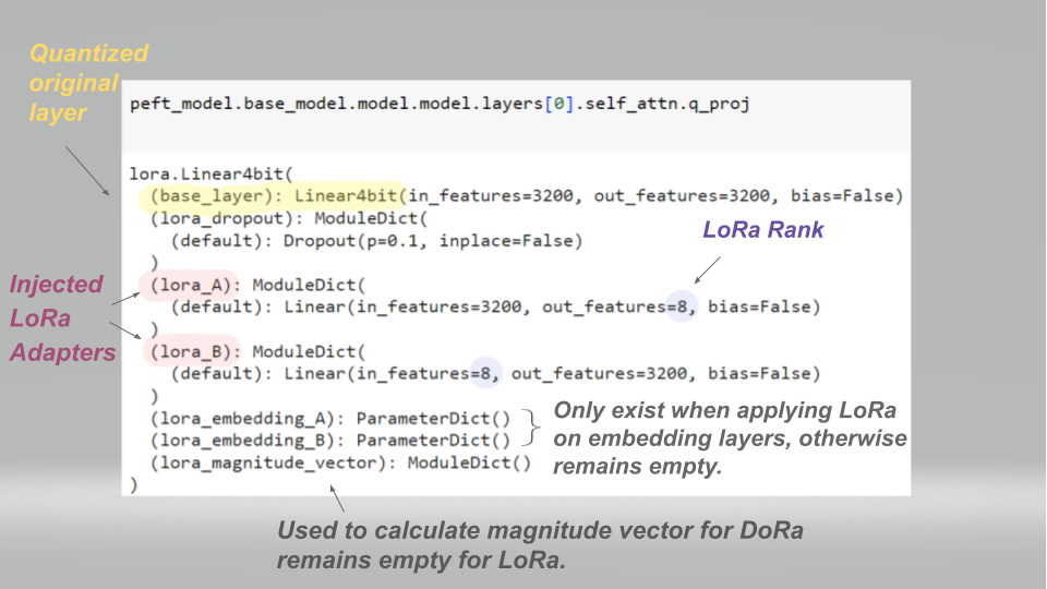
Inspecting W_Q referred to in the model architecture as q_proj, after injecting the adapters into it. Using OpenLLama as quantized base model (hence Linear4bit class) with a LoRa rank of 8 and a dropout of 0.1 — Illustration Created by Author.
This means, ofcourse, that in the backward pass only a smaller set of parameters are updated, that is, fewer gradients to compute and much less optimizer states to maintain compared to full fine-tuning. This leads to faster, more affordable finetuning with less storage requirements.
6. Strategies for Reducing GPU Memory Usage in LLM Finetuning
Besides quantization and LoRa’s efficient finetuning, which are used as memory saving approaches, there are other methods that are currently prevelant in training LLMs. These methods reduce memory consumption without compromising performance and are related to storing activations, gradients and optimizer states during finetuning.
The configuration in the following code contains only the settings that pertain to the important training techniques explained in this section for demonstration purposes, it omits necessary configs related to training like batch_size, learning_rate, etc. Here is a code example with complete configuration.
training_args =  TrainingArguments(output_dir=output_dir,
    gradient_checkpointing=True,
    optim="paged_adamw_32bit",
    gradient_accumulation_steps = 4)

trainer = SFTTrainer(model,
    args = training_args,
    peft_config = lora_config,
    train_dataset = train_data,
    dataset_text_field="input",
    tokenizer=tokenizer)

trainer.train()
Gradient checkpointing — Saving GPU memory by storing less activations.
Gradient checkpointing is a technique used to reduce model memory footprint during backpropagation by storing less activations. Typically in vanilla neural network training, the activations in the forward pass are cached so they can be used in the backward pass to compute the gradients. However for a large model, caching all activations can cause memory overhead. Gradient checkpointing is used to address this issue.
The crux of gradient checkpointing is that instead of storing all activations, we store only a subset of them in the forward pass, mainly the high cost operations that are time consuming, while the remaining ones are re-computed on the fly during backpropagation. This reduces memory usage but it takes longer to complete a backward pass. I believe the name “gradient checkpointing” is somewhat misleading, its alternative name, “Activation checkpointing” seems more appropriate.
You can enable gradient checkpointing by setting gradient_checkpointing to True in TrainingArguments.
Paged optimizer — Saving GPU memory during fine-tuning by moving optimizer states to CPU memory only when GPU memory is fully saturated to avoid out of memory error.
It’s important to note that optimizer states take up a lot of GPU memory, sometimes more than model weights when using stateful optimizers (unlike stateless optimizers like SGD). For instance
AdamWmaintains 2 states per parameter (the first and second moments of the gradient) that need to be stored in memory. This can quickly lead to memory spikes during finetuning. To overcome this issue QLoRa paper introduces paged optimizers.
How does paged optimizers work under the hood?
Paged optimizers use automatic page migration of optimizer states from GPU memory to CPU memory to avoid running out of GPU memory and crash.This technique uses the Unified Memory model introduced in Cuda toolkit 6.0, which provides a single memory space that is directly accessible by CPU and GPU. This technology allows data transfer (page migration) to be automatic in the background using the Page Migration Engine, as opposed to GPU offloading which requires developers to use explicit copy functions to migrate pages between GPU and CPU which is error prone. This effectively prevents OOM error during LLM finetuning. For further reading on Unified Memory with Cuda.
To implement this we set the optim argument to paged_adamw_32bit in TrainingArguments class.
Gradient Accumulation — Saving GPU memory by performing less parameter updates.
Typically in neural network training, a parameter update is performed for each batch. In gradient accumulation, parameter update is performed after multiple batches, this means gradients are accumulated (summed up) for a number of batches before being used to perform a parameter update. However to ensure the magnitude of gradients is within a reasonable range and not too large due to summation, we normalize the loss with the number of accumulation steps.
Furthermore, gradient accumulation simulates training with a larger batch size while actually using smaller batch size. This is because using accumulated gradients over many smaller batches provides more accurate gradient information, which improves the direction of the parameter updates and speeds up convergence. This is similar to what would be obtained from a single large batch, all while avoiding memory constraints that arise with using large batch sizes.
You can enable gradient accumulation by setting the gradient_accumulation_steps argument to greater than 1.
7. Merging LoRa adapters to base model
It’s important to note that during checkpointing, PEFT doesn’t save the entire PeftModel, it only saves the adapter weights which takes up few MB of space. Once the finetuning process is complete, we merge the saved, now trained adapter weights back into their corresponding base layers specified in target_modules of the quantized base model base_NF4_model that we used at the start (you can also merge into the unquantized version of the model). We do this by instantiating a new PEFT model using the base model and the adapter weights, as follows:
# base_dir specifies the directory where the fine-tuned LoRA adapters are stored
lora_model = PeftModel.from_pretrained(model=base_NF4_model, model_id=base_dir)
merged_final_model = lora_model.merge_and_unload()
What does it do?
For each module specified in target_modules, the adapter weights A and B are added to their corresponding original quantized weights.
For instance, \(W_Q\) is updated with the following formula \(W_Q\) = \(W_Q\) + \(ΔW\).
Note that we dequantize the original weight matrix \(W_Q\) from
NF4tobfloat16— the computation dtype we specified inBitsAndBytesConfig— before merging. Dequantization is necessary here to perform the addition operation in higher precision format and maintain as much accuracy as possible.
Here are the exact merging steps :
1.\ Compute \(ΔW\) for \(W_Q\) using its corresponding finetuned LoRa weights A and B as follows:
\(ΔW = A * B * scale\_factor\)
where \(scale\_factor=\dfrac{α}{r}\) as mentioned in the LoRa overview section.
2.\ Dequantize the original weight matrix \(W_Q\) from NF4 to bfloat16 dtype.
3.\ Add the LoRA adapters to the dequantized weight : \(dequantized\_W_Q\) = \(dequantized\_W_Q\)+ ΔW
4.\ Quantize the merged weight back to the original 4-bit quantization with NF4 dtype.
This process ensures that each of the LoRa adapters are integrated into the quantized base model weights efficiently.
LLM Inference Process
Now that we have our quantized models finetuned on our dataset of choice, we can effectively run inference on it (like any other 🤗 model) using the generate() method from 🤗 to produce an output as follows:
inputs = tokenizer(prompt, return_tensors="pt").to('cuda')
with torch.no_grad():
	outputs = merged_final_model.generate(input_ids=inputs['input_ids'])
response = tokenizer.decode(outputs[0])
I bet you guessed the next question : what actually happens during inference to generate our desired response? To answer this question, this section describes the inference process which takes in a prompt as input and generates a response. LLM inference consists of two phases, prefill and decoding :
Prefill Phase of Inference
During the prefill phase, the entire prompt tokens are fed to the model at once and processed in parallel until the first output token is generated.
It’s important to note that we are using a decoder-only based transformer (most common architecture like the GPT model used for next token prediction task) as our code example and the following figure reflects that. Transformer models contain many blocks, but the most important component of the architecture is the masked multi-head causal attention mechanism, which we use during the pre-fill phase. We use masking in this phase (just like in training stage), because we process the entire input sequence at once and we want to prevent the decoder from attending to future tokens and only consider previous ones up to the current token. The figure below summarizes this step:
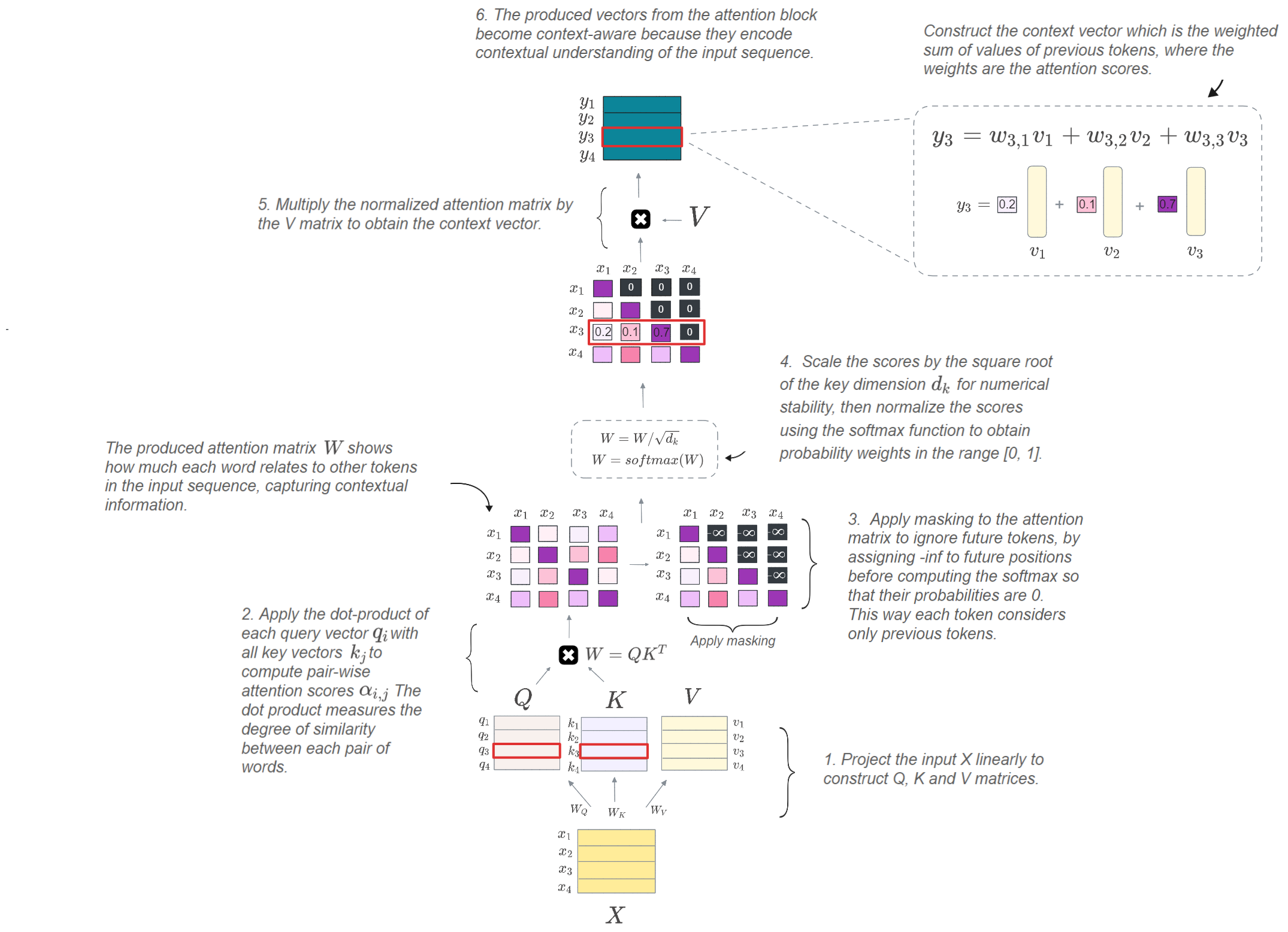
The figure visualizes single head attention with a single sample (not a batch) as input for simplicity. However, transformer-based models currently use multi-head attention (MHA), which allows multiple heads to capture different representations of relationships within the input sequence, resulting in a final representation with a strong contextual understanding of the input — Illustration Created by Author.
If you’re wondering how multi-head attention (MHA) differs from the single-head attention shown in the figure, here’s a short overview: MHA splits the generated Q, K, and V matrices with an assumed size of [batch_size, seq_len, embed_dim] along the
embed_dimdimension intonum_headsparts. This way, each head gets its own set of \(Q\), \(K\), and \(V\) matrices of shape [batch_size, seq_len, d_k] withd_k = embed_dim/num_heads(hence the scaling by d_k in the operation).
However, in practice we use reshaping instead of splitting to apply the scaled dot product (i.e., the attention operation) on a single matrix so that the computation becomes efficiently parallelized. The reshaping is followed by a simple dimension permutation to get \(Q\), \(K\), and \(V\) to have the [batch_size, num_heads, seq_len, d_k] dimension. This way, the same attention operation is computed independently (just like in the figure) to get the weighted sum of values from each head (\(Y\_1\), \(Y\_2\), …, \(Y\_h\)). The final concatenation of the results from all heads is just another tensor reshaping followed by a linear transformation to project the combined context vectors back to the dimenstion of the input \(X\) \([batch\_size, seq\_length, embed\_dim]\).
Here is a corresponding implementation from Karpathy’s mingpt, and here is great post if you want to learn more about multi-head attention mechanism.
Decoding Phase of Inference
The decoding phase contains multiple steps where the model generates tokens one at a time. At each decoding step, the model takes the user prompt coupled with the tokens predicted in previous steps and feeds them into the model to generate the next token.
This phase showcases the autoregressiveness of the model, where it recursively feeds its own output back as input and thus predicting future values based on past values. This process continues until the model generates a special end token or reaches a user-defined condition, such as a maximum number of tokens.
Zooming a bit into the attention block in the decoding phase : At each decoding step, the new token is added to the input sequence, which includes both the user prompt and previously generated tokens. This newely added token attends to all the previously generated tokens through the multi-head attention block where the vector of attention scores are computed using a the scaled dot product.
The scaled-dot product operation in this phase, constructs the query from the new token, while the keys and values are constructed from all tokens. Unlike the prefill phase, no masking is used in the decoding phase because future tokens are not known and have not been generated yet.
GIF shows the reconstruction of K (key) and V (value) matrices using the query and value vectors of previous tokens along with those of the new token, with \(x_4\) as the new token added to the input sequence [\(x_1\), \(x_2\), \(x_3\)]. This means the query vector of the new token will be multiplied with the key matrix K. The result of this dot-product (after scaling and applying softmax) is multiplied by the value matrix V — Illustration Created by Author.
The challenge that arises in the decoding phase is the need to recompute key and value vectors of all previous tokens at each step, resulting in redundant floating-point operations (FLOPs) and slowing down the decoding process.
Optimizing decoding phase with KV Caching
The solution to this is to cache the key and value vectors of each token once they are computed to avoid redundant computations. This cache is referred to as the KV-cache, which significantly speeds up the inference process. The KV-cache is first constructed during the prefill phase for all tokens in the prompt. Then at every decoding step, the cache is updated with the new key and value vectors of the newly generated token, making them the only vectors computed at this step.
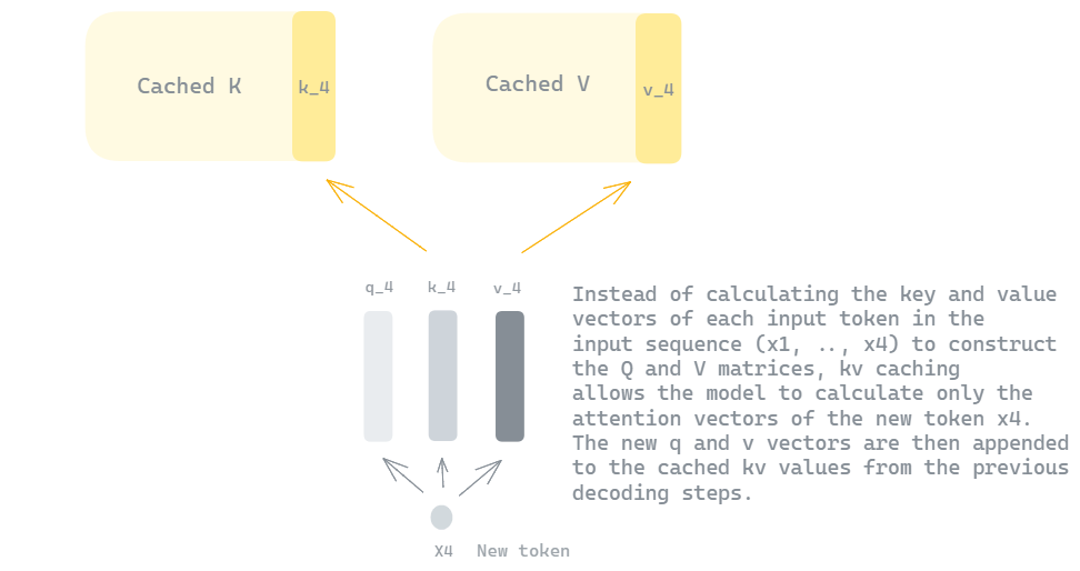
Example of using \(Q\) and \(V\) caches and computing only query, key and value vectors of the new token \(x_4\) — Illustration Created by Author.
In practice, the KV-cache is just a tuple (\(K\_cache\), \(V\_cache\)), where each has the shape \([batch\_size, seq\_len, num\_heads, head\_dim]\), meaning each attention head in the attention mechanism has a separate KV-cache for keys and values.
Here is a code example to demonstrate how both the prefill and decoding phases of inference work when KV-caching is enabled - it uses greedy search decoding for simplicity:
def run_inference(model, tokenizer, prompt, max_length, use_kvcache=True):
    input_ids = tokenizer.encode(prompt, return_tensors='pt')
    kv_cache = (None, None) if use_kvcache else None
    outputs = []
    i = 0
    # prefill phase
    logits, kv_cache = model(inputs_ids, kv_cache=kv_cache)
    next_token = torch.argmax(logits, dim=-1)
    outputs.append(next_token)

    while i < max_length:
        if use_kvcache:
            # only the last input is forwarded to the model
            logits, kv_cache = model(next_token, kv_cache=kv_cache) # update kv_cache
        else:
            # pass the entire sequence (input prompt + generated tokens) to the model
            inputs_ids = torch.cat((inputs_ids, next_token), dim=-1)
            logits, _ = model(inputs_ids, kv_cache=kv_cache)

        next_token = torch.argmax(logits, dim=-1)
        outputs.append(next_token)
        # stop if next_ids is eos token
        if next_token.item() == tokenizer.eos_token_id:
            break
        i += 1

    return tokenizer.decode(outputs)
Here is how the cache would be implemented inside the attention block :
class Attention(nn.Module):
    def attention(self, hidden_states, kv_cache=None, training=False):
        """
        When KV caching is enabled hidden_states correspond only to a single input
        token (which is the last generated token), when it's disabled
        hidden_states correspond to (prompt + generated_tokens_so_far)
        """
        if not training and kv_cache is not None:
            query, key, value = self.linear_projection(hidden_states)
            cached_K, cached_V = kv_cache[0], kv_cache[1]
            # update the cache
            K = torch.cat((cached_K, key), dim=-2)
            V = torch.cat((cached_V, value), dim=-2)
            kv_cache = (K, V)
        else:
            query, K, V = linear_projection(hidden_states)

        atten_scores = scaled_dot_product(query, K, V)
        # we handle any post pocessing of attention scores here
        # to make it ignore certain tokens during attention
        probs = F.softmax(atten_scores)
        attn_output = probs @ V
        return attn_output, kv_cache
Note that we enable KV caching during inference in the generate() by enabling the use_cache flag.
Decoding Strategies
Earlier, we mentioned the greedy search method for selecting the next token, but there are more effective approaches available. Initially, the language model generates a probability distribution over all possible tokens in the vocabulary, the method used to select the next token from this distribution depends on the chosen decoding strategy for text generation.
If you ever had to deal with language model APIs, you may have encountered these methods as configuration options to generate a desired output and you’ll also configure them in the huggingface generate() method we mentioned earlier. Generally, decoding strategies can be categorized into two main classes: maximization based decoding and sampling based decoding.
Maximization Based Decoding
Maximization based decoding selects the next token with the highest probability, that is, it optimizes for model outputs that maximize likelihood. Here are some techniques:
Greedy Search
Greedy search is a simple, naive method that selects the most likely token at each decoding step to construct the final output sequence. However, because it considers only locally optimal tokens it results in low quality, incoherent text.
Beam Search
Beam search is considered a more effective decoding strategy than greedy search, because it’s a search based algorithm that expands the search space at each time step. Instead of simply choosing the single best option at each step like in greedy search, beam search consistently updates of the top K sequences at each step, where K is referred to as the beam width. At the end of the decoding process, we end up with a set of K complete candidate sequences, from which we select the one with the highest probability. As a result, the beam search algorithm is a computationally intensive requiring more model runs than other decoding strategies, because it explores multiple paths by expanding over all selected top k tokens at each decoding step.
However, this decoding strategy performs poorly on open text generation tasks generating repetitive text even when setting a higher beam width.
Beam search might perform well on some NLP tasks with a limited output such as machine translation because it requires a more constrained decoding process that prioritizes accuracy and exact outputs that closely resembles the input. However Beam search doesn’t perform as well on open ended text generation that require more variety in the output. It has been found that language models assign higher probability to tokens with high grammaticality, which when generating longer text, tends to prioritize more generic tokens in a repetitive loop, yielding low quality output — this is referred to as neural text degeneration — Furthermore, human generated text is characterized by diversity, so to make text generation more human like, we use new techniques that introduce randomness into the decoding process to combine likelihood and diversity. This class of techniques is called sampling based decoding.
Sampling based decoding
Sampling based decoding introduce some randomness into the decoding process, which results in a more diverse higher quality text generation. This class includes the following techniques :
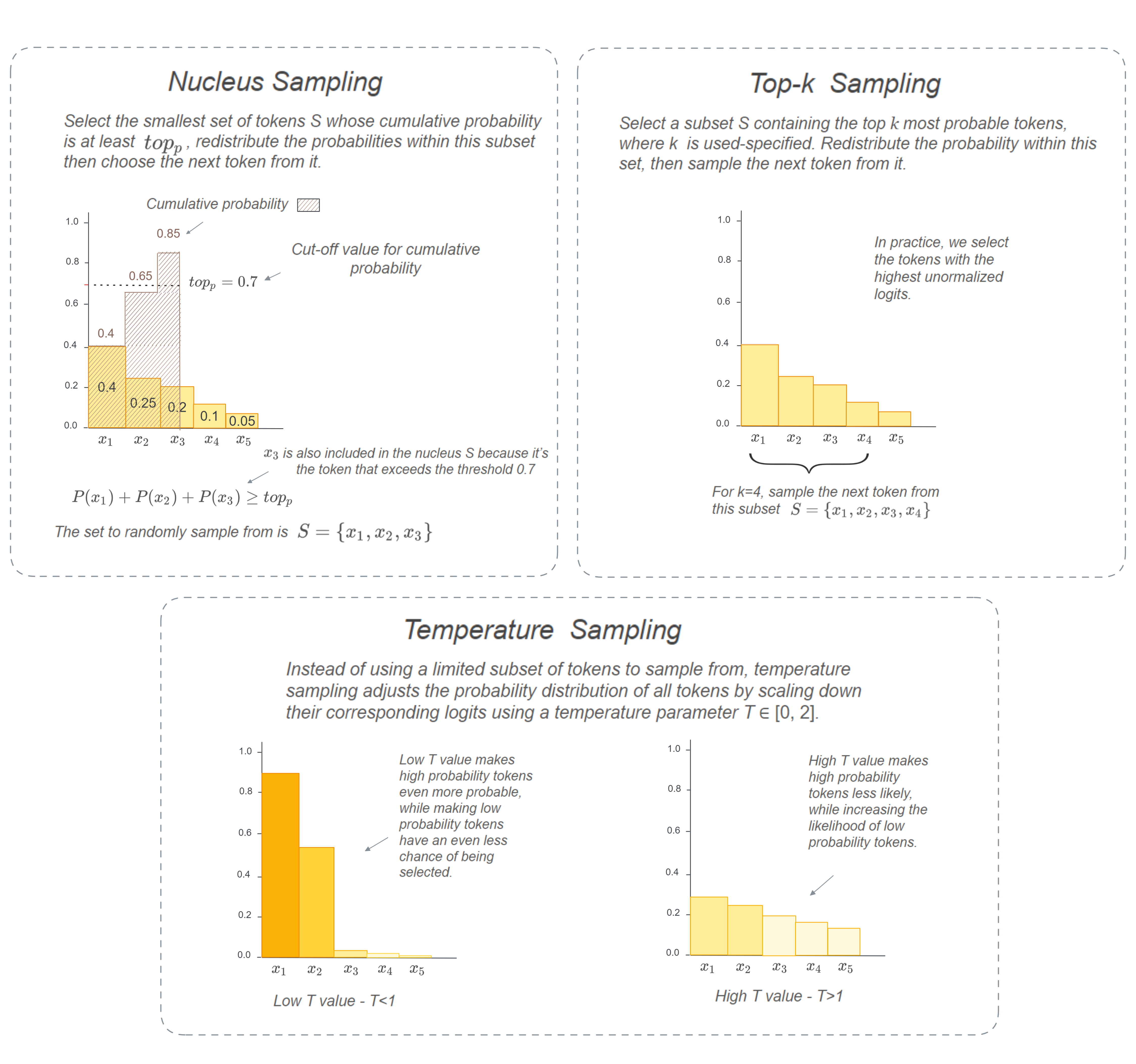
Illustration explaining different sampling decoding methods — Created by Author.
Top-k Sampling
Top-k Sampling introduces randomenss by considering a smaller set of tokens from which we randomly sample the next token from. The chosen tokens are the ones with the highest logit scores, which are unormalized model predictions. This way after applying softmax, the probability distribution is reconstructed and redistributed over this smaller set of candidates, it then samples the next token at random from this new distribution. This approach balances exploring a focused region of highly probable tokens with random sampling. The size of the chosen region is defined by the top_k hyperparameter. Here is the exact algorithm:
-
Select the k highest logits.
-
Set the smallest logit in the top-k logits as a threshold.
-
Keep only tokens with logit values higher than this threshold. In practice, we do not discard the tokens that are below the threshold, we actually assign them a highly negative value (- inf) to ensure that their produced probability after using softmax is exactly 0.
def top_k_sampling(logits, top_k):
    """
    logits [batch_size, vocab_size] : unormalized logit scores.
    top_k : number of tokens to sample from.
    """
    top_logits, _ = torch.topk(logits, top_k, dim=-1) # [batch_size, top_k]
    smallest_in_top_k = torch.index_select(top_logits, 1, torch.tensor([2])) # [batch_size, 1]
    logits[logits < smallest_in_top_k] =  -float('Inf')
    probs = F.softmax(logits, dim=-1) # [batch_size, vocab_size]
    sampled_token = torch.multinomial(probs, num_samples=1) # [batch_size, 1]
    return sampled_token
Although top-k sampling generates a relatively higher quality text with less repetition than beam search, its challenge lies in choosing an appropriate value for the hyperparameter k, because the choice of k depends mostly on the underlying distribution of logits, which varies ofcouse, from one decoding step to another. For instance, it wouldn’t be suitable to sample a small set of tokens from a flat distribution, nor would it be appropriate to sample a large set from a peaked distribution. As result, the following decoding method, “nucleus sampling” mitigates this issue by making the selection of k dynamic.
Nucleus sampling
Nucleus sampling (also referred to as top-p sampling) Instead of having to select a k fixed number of tokens, nucleus sampling dynamically selects the set of tokens to sample from at each decoding step, based on a pre-determined probability threshold \(top_p\) which ranges from 0 to 1.
Nucleus sampling starts by determining the smallest set of tokens whose cumulative probability is at least \(top_p\) such that \(\sum_{i=1}^{k}p_i ≥ top_p\). This set of chosen tokens is analogous to a “nucleus” containing the most probable tokens. Once this set S={\(𝑥_1\),\(𝑥_2\) ,…, \(𝑥_𝑘\)} is determined, it re-applies the softmax function to redistribute the probability over S, and a token is sampled at random from this new distribution (similar to what we did with top-k sampling).
Here is the exact algorithm for further understanding:
-
Apply softmax to generate probabilities over all tokens in the vocabulary.
-
Sort the tokens based on their probabilities in descending order.
-
Include tokens in the final set, starting from the top token with the highest probability, then add the tokens one by one until the cumulative probability of the tokens in this set is at least \(top_p\), that is, we should stop at the token \(x_k\) with a cumulative probability that first exceeds the threshold \(top_p\) . This means we include tokens \(𝑥_1\),\(𝑥_2\) ,…, \(𝑥_𝑘\) in the nucleus S.
-
Set the logits of the tokens not in the nucleus set S to −inf. This effectively removes these tokens from consideration in the next sampling step.
-
Re-apply the softmax function to the modified logits to get the new probability distribution over the nucleus set S.
-
Sample a token from the normalized distribution.
def nucleus_sampling(logits, top_p):
	probs = F.softmax(logits, dim=-1)
	ordered_probs, ordered_indices = torch.sort(probs, descending=True, dim=-1)
	cumulative_probs = torch.cumsum(ordered_probs, dim=-1)

	# create mask of tokens whose cumulative probability is greater than top_p
	# all the False elements including the first True element
	mask = cumulative_probs > top_p

	# include the token that exceeds the threshold - index of the first True element to mask matrix
	indices_to_include = mask.float().argmax(dim=-1, keepdim=True)
	mask[torch.arange(mask.shape[0]).unsqueeze(1), indices_to_include] = False

	# create the new mask with 0s and 1s
	new_mask = mask.float()

	# apply the mask to logits and replace masked out values (0.0) with -inf
	modified_logits = logits * (~ mask) #(1 - new_mask)
	modified_logits = modified_logits.masked_fill(modified_logits == 0.0, float('-inf'))

	# Map the modified logits back to the original order
	template = torch.zeros(logits.shape)
	final_logits = template.scatter(1, ordered_indices, modified_logits)

	# repass the logits back to softmax
	probs = F.softmax(final_logits, dim=-1) # [batch_size, vocab_size]
	sampled_token = torch.multinomial(probs, num_samples=1) # [batch_size, 1]
	return sampled_token
Here is the huggingface implementation.
A smaller
top_pvalue considers only the highly probable tokens for sampling, with fewer tokens to choose from the generated text is less creative. Meanwhile a highertop_pvalue results in a more varied and creative output, with the potential risk of generating semantically incoherent text.
Temperature Sampling
Temperature Sampling is a calibration method that scales down the unormalized logits using a hyperparameter T which ranges between 0 and 2, before passing them to the softmax function.
The generated predictions can sometimes be naive, in that, it could produce very peaked probability distribution that results in over-confident predictions for few tokens. To address this, we calibrate the distribution to adjust model confidence by introducing a degree of randomness using temperature. Then as usual with sampling methods, we sample at random from the resulting probability distribution:
scaled_logits = logits / temperature
probs = F.softmax(scaled_logits)
-
Using a high T value
T>1results in a flatter distribution, where most tokens across the range are probable. This less confident probability distribution leads to a language model output generation that is more stochasitc and creative (though this is not always case). -
Using a low T value
T<1produces a peaked distribution making previously high-probability tokens even more probable. This confident probability distribution leads the language model to generate more consistent deterministic response.
These sampling techniques can be combined together by modifying the probability distribution sequentially, starting with temperature sampling followed by the sampling methods. This ensures that the selected set of tokens have non-zero probabilities while zeroing out the probabilities of tokens that do not belong to this set. We then randomly sample the next token from the produced distribution using the
torch.multinomialsampler, which is not to be mistaken with whatnumpy.random.choicedoes with uniform random sampling — I used numpy as an example because the equivalent operation in Pytorch is not as straightforward —torch.multinomialsamples from the input tensor with or without replacement (when using n>1), ensuring that the selection takes into consideration the probabilities assigned to each token, with tokens having higher probabilities being more likely to be chosen.
Now that we understand what each strategy achieves in tuning the desired LLM response, the recommendation is as follow: you’d want to increase randomness to encourage exploration and diversity in generated text for creative tasks like storytelling (configure higher values for T | top-k | top-p). However excessive randomness can lead to meaningless outputs. Meanwhile too little to no randomness leads to a more predictable and consistent outputs, which is useful for tasks that require precise and consistent responses like machine translation (decrease T | top-k | top-p) but might cause the model to repeat itself or generate very generic responses.